NNadir
NNadir's JournalDiagramming making bad coffee.
I was reading a paper today, this one, Development and Optimization of Liquid Chromatography Analytical Methods by Using AQbD Principles: Overview and Recent Advances and I came across a reference to a "Ishikawa Fishbone Diagram."
We are fortunate in these times that when we don't know what something is, we can google it, and often end up at Wikipedia, which is what happened to me, where I learned how to make a diagram of how I might make bad coffee:
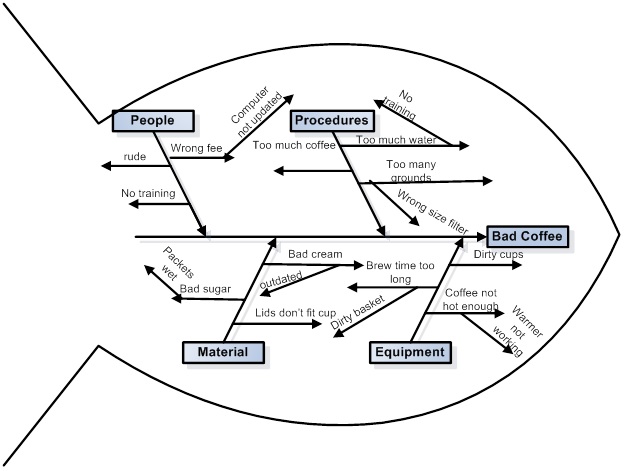
Feel free to follow these steps to making bad coffee.
It turns out that I've seen these types of diagrams before, but never knew what they were called. Now when I'm in a meeting, I can say "Ishikawa Fishbone Diagram" and sound like I know something, even if I don't know shit from shinola.
I was mistaken about the timing and magnitude of the 2019 Mauna Loa CO2 minimum.
On September 22 I wrote the following in a post in this section:
This year, in 2019, as is pretty much the case for the entire 21st century, these minima are uniformly higher than the carbon dioxide minima going back to 1958, when the Mauna Loa carbon dioxide observatory first went into operation. Weekly data is available on line, however, only going back to the week of May 25, 1975, when the reading was 332.98 ppm.
For many years now, I have kept spreadsheets of the data for annual, monthly, and weekly Mauna Loa observatory data with which I can do calculations.
In the weekly case, the week ending May 12, 2019 set the all time record for such readings: 415.39 ppm.
These readings, as I often remark vary in a sinusoidal fashion, where the sine wave is imposed on a monotonically increasing more or less linear axis, not exactly linear in the sense that the slope of the line is actually rising slowly while we all wait with unwarranted patience for the bourgeois wind/solar/electric car nirvana that has not come, is not here and will not come.
This graphic from the Mauna Loa website shows this behavior:

Here is the data for the week beginning on September 15, 2019
Up-to-date weekly average CO2 at Mauna Loa
Week beginning on September 15, 2019: 408.50 ppm
Weekly value from 1 year ago: 405.67 ppm
Weekly value from 10 years ago: 384.59 ppm...
...The operative point is that this reading is only 0.09 ppm lower than last week's reading, which was, 408.59 ppm. This suggests, if one is experienced with working with such data, that this is most likely the annual September minimum reading. For the rest of this year, and through May of 2020 the readings will be rising. We will surely see next May readings around 418 ppm, if not higher.
However, I was wrong, because the next two weeks at Mauna Loa showed values lower than 408.50 ppm. It actually took place this year during the week ending 09/29/19, when the reading was: 407.97
The most recent data point is the week ending October 6, 2019 is a follows:
Up-to-date weekly average CO2 at Mauna Loa
Week beginning on October 6, 2019: 408.39 ppm
Weekly value from 1 year ago: 405.50 ppm
Weekly value from 10 years ago: 384.06 ppm
Last updated: October 13, 2019
From here on out, until May, 2020, the values for each week will exceed the number reported on September 29 of this year.
Previous weekly data annual lows took place as follows over the last 5 years:
9/9/18: 405.39 ppm
9/24/17: 402.77ppm
9/25/16: 400.72ppm
9/27/2015: 397.2 ppm
9/14/2014: 394.79 ppm
No one alive today will ever see a measurement at Mauna Loa lower than 400 ppm again.
In 2000, the weekly data annual low took place on September 10, 2000: 367.08 ppm.
In 1980, the weekly data annual low took place on September 4, 1980, 339.87 ppm.
In 1975, the first year the weekly data was reported, the weekly data annual low took place on August 31, 1975 when it was 329.24 ppm.
The movement to late September is most probably a function of a warmer and longer summer in the Northern Hemisphere, during which the annual minimums take place.
The annual maxima show up in early May. We may expect that the 2020 maximum should approach or exceed 418 ppm.
I apologize for jumping the gun. It's possible that next year we'll see, for the first time ever, the minimum appearing in October.
Have a nice afternoon.
The amplitude and origin of sea-level variability during the Pliocene epoch
The paper I'll discuss in this post is this one: The amplitude and origin of sea-level variability during the Pliocene epoch (Grant et al, Nature volume 574, page s237–241 (2019).
This past Thursday I posted a similar paper about this epoch, which was also published in Nature, in the same issue, just above this one.
During the Pliocene Epoch, which was from 3 to 5 million years ago, the concentration of carbon dioxide in the atmosphere apparently surged (for a few hundred thousand years) to around 450 ppm, which, since we are doing nothing meaningful about climate change, we will hit in about 15 to 20 years.
The authors here use a different approach than the approach I discussed on Thursday.
From the abstract:
The authors review, as the authors described in my previous post, the techniques for evaluating the sea level in the geological past:
...and describe some significant limitations, for example with the ?18O method...
They then describe their approach:
Reference 6 is this one, from the same group:
Mid- to late Pliocene (3.3–2.6 Ma) global sea-level fluctuations recorded on a continental shelf transect, Whanganui Basin, New Zealand (Grant et al Quaternary Science Reviews Volume 201, 1 December 2018, Pages 241-260) I have not personally accessed this paper.
A few more details on their approach:
Some pictures from the text:
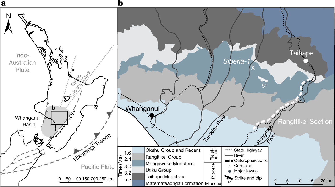
The caption:
 ?as=webp
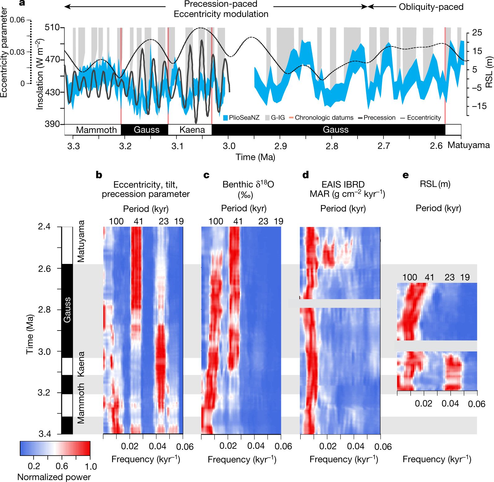
The caption:
The caption:
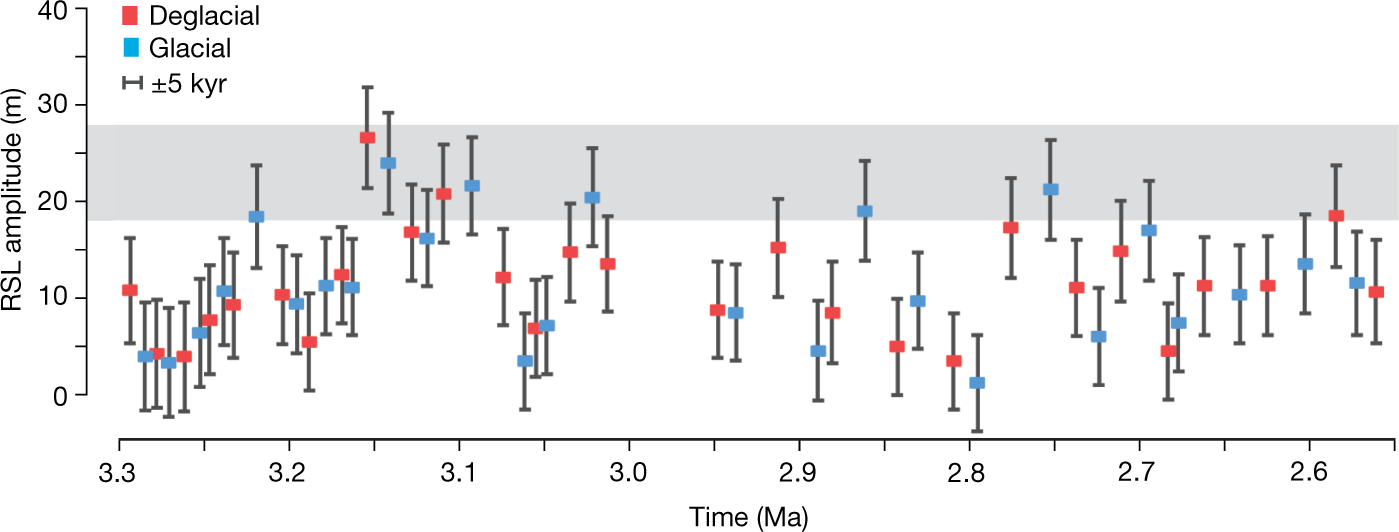
https://www.nature.com/articles/s41586-019-1619-z/figures/4
The caption:
AIS is the antarctic ice sheet, GIS, greenland ice sheet.
They speak on the effect of rotational precession changes the insolation patterns drive this historical warming, and that this in turn, they argue, means that the Antarctic Ice Sheet is more prominent in driving sea level rises.
This does not mean that they exclude carbon dioxide, far from it.
From their conclusion:
Have a pleasant Sunday afternoon.
A Tale of 2 Radioactive Contamination Issues: the San Joaquin Oil Fields & Fukushima Seaweed & Tuna.
The two papers I will discuss in this post are from a recent issue, as of this writing, of one of my favorite scientific journals, Environmental Science and Technology.
They are:
Occurrence and Sources of Radium in Groundwater Associated with Oil Fields in the Southern San Joaquin Valley, California (McMahon et al, Environ. Sci. Technol. 2019, 53, 9398?9406.
...and...
Temporal Variation of Radionuclide Contamination of Marine Plants on the Fukushima Coast after the East Japan Nuclear Disaster (Arakawa et al Environ. Sci. Technol. 2019, 53, 9370?9377)
I will also briefly discuss, in papers linked below, the famous Fukashima Tuna Fish.
The second paper is behind a firewall but may be accessed in an academic library; the first is open sourced and anyone can read it.
For convenience I will treat them both as if they were behind a firewall, and excerpt portions and graphics of both.
Before launching into a discussion of the papers, it is worthwhile to discuss the nuclear properties of all the species discussed in the paper. To do this, I will provide references to other papers as well as links to those that have them. These papers have largely been downloaded or scanned into my personal files but many, if not all, may be accessed in a good academic library.
Almost all of the data in the discussion of the nuclear properties here were sourced from the website of the National Nuclear Data Center by entering the symbol for the nuclides in question in the top box and clicking the "decay data" in the right hand box. This will lead to other links, where one can use the "human readable" form to get the information on half-lives and decay energies. This data can also be accessed using the "periodic table browse" tab.
The radioactive nuclides discussed in the first paper are all anthropogenic nuclei created in the operation of nuclear reactors, two isotopes of cesium-134 (Cs-134), and cesium-137(Cs-137). The latter is a fission product. The former is formed by neutron capture in non-radioactive cesium-133, also a fission product. (The direct formation of cesium-134 does not take place since Xenon-134, a fission product preceding it is observationally stable and thus not subject to measurable radioactive decay.) Also discussed is an isotope of silver, silver-110m (Ag-110m), a nuclear isomer of radioactive silver-110 (Ag-110). Cs-134 has a half-life of 2.06 years. Cs-137 has a half-life of 30.08 years. Ag-110m has a half-life of 249 days, roughly.
It has been roughly 3100 days since the last reactor at Fukushima suffered a hydrogen explosion. The fraction of Ag-110m that remains is about 0.000178 of that which was present when the explosions took place, and, as silver chloride is insoluble, I will not discuss this isotope at any length in this post even though it mentioned in the paper on Fukushima to be discussed. It is however discussed in the paper as a kind of marker, despite it's extremely low concentrations.
The decay energy of Cs-137 is nominally 594 keV, however most of this energy is carried off as a neutrinos with a mean energy of 370 keV. As neutrinos interact only weakly with matter there is little effect on matter, living or dead. Most of the energy that does interact with matter is in the form of a ?- particle, with a mean energy of 179 keV. Beta particles are not particularly penetrating, but can damage local matter when it decays, including living tissue if it is in contact with it or internalized in it.
Cesium-137 is, however, responsible for two nuclear decays, that of itself, and that of its daughter, Ba-137m, the nuclear isomer of stable Ba-137. Since the half-life of Ba-137m is 2.55 minutes, Cs-137 is in secular equilibrium with Ba-137m, which emits a 594 keV gamma ray in its isomeric transition, under most conditions. Since the decays are quite nearly simultaneous on an effective transport time scale, this gamma ray is sometimes reported as the decay energy, which is 661 keV (0.661 MeV) of cesium although it is actually a decay in barium. The concentration of Cs-137 is thus often determined by the secular equilibrium ratio by detection of this Ba-137m gamma ray. Gamma rays can interact strongly with matter by breaking chemical bonds, even strong bonds, for example carbon-fluorine bonds. They also can easily break bonds in living tissue, which is why they can kill cells, and in high enough doses, whole organisms including human beings.
Barium-137m can be placed in disequilibrium by exploiting the insolubility of barium carbonate or sulfate. Cesium sulfate and/or carbonate are completely soluble. If disequilibrium occurs, and the mixture is not subject to additional active separation, equilibrium represented by the maximal accumulation of Ba-137m is reestablished in about 57 minutes.
(I often reflect on this disequilibrium when considering certain kinds of radiocesium hyroxide devices for storing (and/or converting) decay energy for work utilizing compressed air, since a side product of the scheme would be air capture of carbon dioxide and the destruction of certain kinds of problematic long lived greenhouse gases that have been released into the atmosphere by the refrigeration industry.)
Cs-134, the other radioactive cesium isotope released in significant quantities at Fukushima, decays directly to stable Ba-134. It has a decay energy of 2,058 keV (2.058 MeV), much of it released in the form of an gamma rays with an average energy of 1558 keV (1.558 MeV) It decays almost exlusively by ?- emission; the average energy of the ?- particle is 157 keV.
Ag-110m largely decays directly to cadmium-110. It has a decay energy of 2,968 keV (2.968 MeV). Most of it decays by ?- emission, with an average(? emitter, HL seconds, decay energy, keV ( MeV)) particle energy of 67 k and a gamma ray with an average energy of 2,760 keV, (2.76 MeV). A small amount (1.36%) decays to Ag-110, which has a half-life of around 24 seconds and a similar energy to the parent 110m nuclear isomer.
All three of these isotopes, Cs-137, Cs-134 and Ag-110m were released by the meltdown of the Fukushima reactors.
The paper discusses the fate of these isotopes in seawater and in seaweed in the general Fukushima area, as well as their relative concentrations.
The radioactive species discussed in the second paper are all called Naturally Occurring Radioactive Materials (NORM). It is chiefly concerned with two of these, radium-226, a part of the uranium-238 decay series, and Radium-228, a part of the thorium decay series. Both are highly energetic alpha emitters. Ra-226 is the parent isotope of 9 (or more, depending on branch ratios) additional nuclear decays. Ra-228 is the parent leading to 10 additional nuclear decays.
The half-life of Ra-226 is 1600 years. The half-life of Ra-228 is 5.75 years.
The decay energy of Ra-226 (? emitter, HL 1600 years, decay energy, 4,871 keV (4.871 MeV)) is almost an order of magnitude higher than the decay energy of Cs-137, the longest lived, and in many ways the most problematic of all fission products. The daughter nuclides of the decay of Ra-226 are these, with "Half-life" abbreviated "HL:"
Rn-222 (? emitter, HL 3.8235 days, decay energy, 5,590 keV (5.590 MeV)),
Po-218(? emitter, HL 3.098 minutes, decay energy, 6,114 keV (6.114 MeV)) (minor 0.02% ?- ),
Pb-214 (?- emitter, HL 26.8 minutes decay energy, 1,019 keV (1.019 MeV)),
Bi-214 (?- emitter, HL 19.9 minutes decay energy, 3,270 keV (3.270 MeV)) ,
Po-214(? emitter, HL 164.3 ?seconds, decay energy, 7, 833 keV (7.833 MeV)) ,
Pb-210 (?- emitter, HL 22.2 years decay energy, 63.5 keV (0.0635 MeV)) ,
Po-210 (? emitter, HL 138.376 days, decay energy, 5,407 keV (5.407 MeV)),
Pb-206 (stable)
The reason for producing these details is to show that the energy associated with the decay of radium is much higher than the energy associated with the decay of the radioactive cesium isotopes. If this energy is deposited in living tissue the matter is more serious.
The effects of radiation on tissue is the subject of efforts to systematize it as so as to make reasonable assessments of risk; a considerable effort has been made which is probably very good to a first approximation to produce something called “quality factors” which is a function of the type of radiation, in most cases here alpha radiation, which is not very penetrating and thus deposits most of its energy locally, the type of tissue and the density of the tissue in which it traveling. This is the type of thinking that goes into the unit “Sievert,” abbreviated “Sv” which is frequently a unit mentioned with respect to the health risks of radiation. It has replaced the “Rem” in common radiation health, and accounts for the type of radiation.
A related unit is the “Gray” which is a measure of the amount of energy deposited in a material, which is also a function of the nature of the material, extending beyond tissue. The Gray involves less subjectivity than the Sievert.
The total amount of energy generated by the decay of radium and it’s daughters, in their decay is a whopping 34,186 keV. Since much of this energy is in the form of low penetrating ?- and ? particles, it follows that much of it is in fact deposited in tissues if the nuclide is internalized in the tissue.
The unit keV is an atomic unit and may not mean much to the average citizen not accustomed to dealing with such units. The conversion factor between this unit and the more familiar energy unit the Joule is simply the charge on an electron, 1.609 X 10^-19 Coulombs times 1000 to account for the “k” from kilo-. It is useful to consider how much energy a gram of “radium daughters.”
Of the above nuclei listed in the radium decay series, the one with the shortest half-life that is actually long lived enough to have actually been isolated is Po-210. This is the nuclide that Vladmir Putin’s agents utilized to kill the renegade Russian Security Agency Defector Alexander Litvinenko. (All of the world’s commercial Po-210 is manufactured in Russia and is exported to countries around the world to control static in the manufacture of very sensitive microcircuits for example.) Therefore to consider how much energy a “MeV” is, let’s take a look at the macroscopic energy output of a gram of this element’s isotope puts out. Using the conversion factor from the previous paragraph, we see that the decay of a single atom of Po-210 puts out .870 nanoJoules of energy, or 870 picoJoules.
The number of atoms decaying in a second is given by the specific activity of Po-210, which is in turn, determined by its decay constant, ?, which is defined by dividing the natural logarithm of 2 by the half-life in seconds, which in the case of Po-210, works out to 5.80 X 10^(-8) inverse seconds. Multiplying this number by Avogadro’s number gives the number of decays in a mole of Polonium-210, and dividing it by the approximate atomic weight of Po-210, 210, gives the number of decays per second. This number is 2.5 trillion decays per second per gram. Multiplying this by the decay energy, we see that a gram of Po-210 puts out about 2,170 watts of power.
The density of the beta phase of polonium, which is the only phase that can be reliably measured given the heat output of the metal, is about 9.4 g/ml, meaning that the volume of a gram is simply the inverse of this number or about 0.11 ml. A teaspoon is said to be 9.2 ml, and it follows that a gram of polonium-210 putting out 2,170 watts is about 0.02 teaspoons.
It is the high energy to mass ratio that makes nuclear energy environmentally superior to all other forms of energy.
However, as is clear from the Litvinenko case, ingesting or being injected, even in amounts much less than a gram, of Po-210 will kill a person.
Much of what I have written above is misleading, in the sense that it implies that if one were to eat radium, or to drink it in well water contaminated with it – the possibility of which is discussed in one of the papers, to be discussed herein – one would be subjected to all of the decays during one’s lifetime, which is decidedly not true. A “bottleneck” in the decay series is the relatively long half-life of lead-210. The radioactive elements in a decay series are subject to various kind of equilibria, and the equations of radioactive decay, derived from the Bateman Equation.
From the use of these equations, it can be shown that the attainment of transient equilibrium between Ra-226 and Pb-210 would take about 139 years to achieve, at which time the ratio between the parent nuclide (Ra-226) and the daughter (Pb-210) would be 0.0139. Moreover the equilibrium ratio of Pb-210's daughter, Po-210, to Pb-210 would be 0.017, meaning that the ratio of ratio of Po-210 to Ra-226 would be 0.00027 or 0.027%. Only 94.2% of the radium originally present would remain at this point.
This is why Marie Curie was not immediately killed by isolating radium; it took a long time to reach Po-210 equilibrium. In fact, it took 36 years for her work with radium (and other radioactive elements) to kill her, a period of remarkable scientific achievement during which she was awarded two Nobel Prizes. (She and her husband had previously isolated tiny amounts of Polonium, before their discovery of radium, from uranium ores, but not enough to kill them; the amounts were invisible, and in fact, still shielded by significant quantities of uranium.
But let’s be clear, her work with radioactivity did kill her.
Nevertheless, people do regularly consume polonium, at least to the extent they eat seafood.
The ocean contains about 4.5 billion tons of uranium, albeit in low concentrations, a generally accepted average level being around 3.3 ?g per cubic meter, although this figure can vary from place to place. In the Mediterranean Sea, for example, measurements of concentrations of uranium in seawater ranged from between 3.2 to 3.7 ppb, (XAS and TRLIF spectroscopy of uranium and neptunium in seawater Melody Maloubier, et al Dalton Trans., 2015,44, 5417-5427), between 3.01 and 3.15 ppb in the anoxic Saanich Inlet, a fjord on Vancouver Island in Canada (Uranium isotope fractionation in Saanich Inlet: A modern analog study of a paleoredox tracer (C. Holmden et al. Geochimica et Cosmochimica Acta 153 (2015) 202–215) and fairly precise measurements in the seas around Tiawan gave 3.116 ppb with a relative error of around 1.6%. Measurements of natural uranium concentration and isotopic composition with permil‐level precision by inductively coupled plasma–quadrupole mass spectrometry (Shen et alGeochem. Geophys. Geosyst., 7, Q09005, )
Uranium in seawater has been there ever since the Earth's atmosphere began to feature significant concentrations of oxygen, for billions of years. It has thus had plenty of time to come into transient equilibrium with its daughter radium. It takes "only" 34,282 years for this equilibrium to be established. Although radium carbonate and radium sulfate have low solubility products, they are high enough that disequilibrium is not obtained commonly in seawater; it is estimated that the scavenger lifetime of radium in seawater is six times longer than its radioactive half-life. (cf Teh-Lung Ku and Shangde Luo, U-Th Series Nuclides in Aquatic Systems, Cochran and Krishnaswami, ed. Ch 9 pg 313).
It follows that seawater naturally contains Po-210, and, it turns out, organisms concentrate this polonium.
A rather famous paper in the scientific literature, famous mostly for the idiocy which the international media interpreted it, concerns the "Fukushima Tuna Fish." The paper is here: Pacific bluefin tuna transport Fukushima-derived radionuclides from Japan to California (Madigan et al PNAS 109 24 9483–9486 (2012)). The purpose of the paper was to utilize a particular marker, the relatively short-lived nuclide Cs-134, that was injected into the sea by the destruction of the Fukushima nuclear reactors by a natural catastrophe to trace the migration of tuna and not to publicize a huge health risk.
However, because of the publicity the paper generated, the embarrassed authors felt to publish a follow-up paper, Evaluation of radiation doses and associated risk from the Fukushima nuclear accident to marine biota and human consumers of seafood (Madigan et al PNAS 110 26 10670–10675 2013).
They wrote:
More than 1100 newspapers...
The journalists engaged in this reporting remind me of a really, really stupid guy who made it to my ignore list here who once represented that the collapse of a tunnel at the Hanford Reservation, which turned out to contain some slightly radioactive discarded chemical reactors, was somehow more important than the complete destruction of the planetary atmosphere by dangerous fossil fuel waste.
No wonder ignorance is accelerating climate change. There are actually people who think we cannot use the nuclear tool – the only tool which has worked on a significant scale – to address, slow, and perhaps even halt, the ongoing destruction of the entire planet’s atmosphere because some fool on a Trumpian intellectual level heard about a small tunnel with some rail cars in it with old chemical reactors contaminated with a small amount of residual plutonium. One hears these kinds of things, but one really doesn’t want to believe it.
As for the tuna fish, the weighted absorbed dose from the radiation from natural Polonium-210 in the "Fukushima Tuna Fish" was found to be 558 ?Sv from Polonium-210, 12.7 ?Sv from the natural radioactivity associated with potassium (K-40) - both tuna fish and humans would die without mildly radioactive potassium - 0.5 ?Sv from Cs-137, most of which resulted from nuclear weapons testing in the 20th century, and 0.4 ?Sv from the Fukushima Cs-134 that was being utilized to track the tuna fish migration patterns.
What is interesting in terms of actual radioactive decays, the number of decays attributed to Cs-134 in a kg of dry "Fukushima Tuna" is 4 Beq, and Po-210 only about 20 times larger, 79 Beq, as compared to the factor of risk as measured in ?Sv, which is almost 1400 times higher for Po-210 with respect to Cs-134, although these risks are almost vanishingly small in any case. Very few people get radiogenic cancer from eating the polonium in a kg of tuna fish. The radiation associated with a tuna fish is a fraction of normal background radiation and, in fact, if the tuna has spent a significant time in a can, most of the polonium will have decayed away to lead.
The point here, of all the diversion, is simply – an issue addressed by the unit “Sievert” – is to reify the fact that in terms of health, the issue is not how many decays a radioactive substance undergoes and also where it is located. A committed dose represents an ingested radionuclide, Polonium from a tuna fish for example.
The biochemistry of the radioactive elements is also very important in determining risk. The measured concentration of natural polonium in seawater is rather low, a Malaysian paper on the subject describing what the authors regard as high concentrations of the element reports concentrations of Polonium in seawater that is orders of magnitude lower than what the exasperated authors of the "Fukushima Tuna Fish" paper reported in the fish. (High 210Po Activity Concentration in the Surface Water of Malaysian Seas Driven by the Dry Season of the Southwest Monsoon (June–August 2009) (Sabuti, A.A. & Mohamed, C.A.R. Estuaries and Coasts (2015) 38: 482). This is because polonium - although a metal or semi-metal - is technically chemically a cogener of oxygen and sulfur and thus can behave like these elements. Squid also concentrate polonium, and the authors of a paper discussing the radiological effects of squid consumption in Korean and Portuguese diets. (Distribution patterns of chalcogens (S, Se, Te, and 210Po) in various tissues of a squid, Todarodes pacificus (Kim et al Science of The Total Environment 392, 2–3, 25 2008, 218-224.
The behavior of polonium as a chalcogen suggests its utility in medicine. Radiation kills cells and cells that we would like to kill are cancer cells. A particular type of antineoplastic drug that is becoming increasingly subject to research is an "ADC" - an antibody drug conjugate - in which an antibody with an affinity for cancer cells is linked to a "payload," a toxic antineoplastic drug, for example pacitaxel or vincristine. Radioactive substances like technetium can also be utilized in this way, but generally the linker is not part of the antibody structure, but is rather an introduced complexation agent, introducing issues with stability and selectivity for cancer cells. (The idea behind most medicinal chemistry approaches to cancer is to use a cell cancer killing agent which will kill more cancerous cells than healthy cells, but healthy cells are invariably killed.
When I was a kid, for a while I was working on the synthesis of selenols and tellurinols of aromatic species to model certain biological enzyme behavior, and my adviser joked that perhaps we should extend our efforts to include "poloninols." It was a joke, but actually one can imagine, should this be synthetically feasible, incorporating polonium into tyrosine, cysteine or methionine residues in proteins to make a cancer cell targeting antibody that carries polonium directly into a tumor and is filtered from the blood stream by the tumor, killing it. Whether someone has explored this option, I do not know. It would be interesting to know the chemical form of polonium in tuna fish, for example if it exists in the form of polonocysteine, for example, and perhaps this has been investigated, I don’t know.
A last diversion before turning to the papers I promised to discuss at the outset:
At the outset of this post, I disingenuously suggested that the decay energy of the entire radium series would be 34,168 keV (34.1MeV). I then went on to explain that in fact, there are decay “bottlenecks” which prevent all of this energy from being deposited in entirely in a person experiencing a radium decay in their flesh, most notably the existence of Pb-210 in equilibrium with its daughter Po-210. Nevertheless, in the case where a parent nuclide decays with a much longer half-life than it’s daughter(s), it is common practice to consider the case, to a first approximation, as if the decays are effectively simultaneous, as one does in determining the presence of Cs-137 from the Ba-137m gamma ray. The half-life of radium is sufficiently longer than all of its decay daughters up to Pb-210 so that it is pretty much possible to do this, but if one lives for decades after ingesting the radium – and people do this, as evidenced by the life of Marie Curie – only a portion of the energy from the decay of Pb-210 will be available to damage living cells. The total decay energy of radium and all of its daughters up to and including Po-214 is 28,697 keV (28.6 MeV), an enormous amount of energy on a molecular scale.
Here too, however, there is a caveat. The decay series of Ra-226 through Po-214 contains, the longest lived nuclide among them, gaseous radon-222. When deciding whether all of this energy in this decay series is deposited in flesh when an atom of radium decays, one must account for this fact, the chemical nature of radon, which is an inert noble gas.
It is well known that radon gas is associated with lung cancer. Radon gas is present wherever there is a uranium formation is present; for example, I live over the Reading Prong uranium formation and I have measured radon in by basement, where, in fact, I am writing this post. Happily for me, the concentration of this radon is below what is considered an action level.
Many mass market/popular books have been written on the subject of lung cancer among Native American uranium miners who worked in the mid-20th century and their lung cancer rates, which are significantly higher than among control populations. With appeal to some published scientific literature on this case – there is a great deal of that too, besides the popular books – as well as the popular books, I have written on this subject myself elsewhere on the internet. An excerpt:
Sustaining the Wind Part 3 – Is Uranium Exhaustible?.
There won’t be a lot of books written about the 19,000 people who will die today from the dangerous fossil fuel and biomass combustion waste called generically “air pollution,” nor many shut by the health risks of the Native American coal miners in the same general region who lost their jobs this year, but that to which we pay attention says a great deal about who we are.
It is generally understood that the risk of breathing radon gas are associated with the decay daughter discussed above, including, but not limited to polonium-210 and its parent, lead-210. It is the case, however, that the physiology of radon is not quite as simple as being inhaled and exhaled in a passive manner so that the risk is associated with a series of cases where radon atoms decay while in the lungs, depositing radioactive polonium, bismuth or lead.
For one thing, radium, radon’s parent, is, like the fission product strontium, deposited in bones, as it is a cogener of calcium and, like strontium and barium, behaves very similarly to it. Thus it is relatively easy for radon gas to be trapped in this dense matrix, much as radon gas, and for that matter helium gas – all of the world’s helium is derived from atoms once trapped in rock – to be trapped in bone. Much of the energy of alpha decays appears initially as high energy recoils. An alpha particle emitted at a few MeV is traveling at relativistic speeds, that is, a significant fraction of the speed of light, and it follows that the conservation of momentum will result in the daughter nuclei formed in the decay also traveling significant distances in the material it damages. This is well known in rock. If the rock is ground into fine particles, as in a fracking operation, these particles may be propelled to the surface of the particle or beyond it. Most oil and gas (and for that matter coal) deposits were formed by the reformation of biomass over hundreds of millions of years and deposited in sedimentary rocks (or possibly metamorphic) rocks. If the formations formed from oceanic deposits, they will contain oceanic uranium, in some cases concentrated by organisms – coral, for one example, greatly concentrates uranium from seawater – or, if formed terrestrially in lakes or in forests, will form from the uranium ores weathered. Thus these formations typically have uranium impurities in them, and thus uranium daughters.
It is true that radon can travel via recoils several millimeters in bone, and thus radium deposited near the surface of the bone can propel radon atoms out of bony tissue into other tissues. Theoretically, one would think, this would make the radium be solvated in the blood stream and possibly be transferred into the air via exhalation through the lungs.
It is not, however, quite that simple.
Naively, assuming that radon behaved much like xenon, krypton and argon, I rather thought that radon would be appreciably soluble in water via the formation of clathrates, and to some extent this is true. A nice open sourced discussion of radon clathrates and their association with the migration within uranium bearing soils is found here: The origin and detection of spike like anomalies in soil gas radon time series. (Chyi et al Geochemical Journal 25 431-438 (2011))
The idea of radon clathrates suggests that for whatever reason, something rather like hydrogen bonding, radon is hydrophilic.
The behavior of radon in tissue has been studied and a number of interesting papers on the subject have been published, using both animal and human subjects. A very recent paper on the subject explores the theoretical justification for the observed fact that physiologically, radon tends to have an affinity for hydrophobic lipids, that is fat tissue. The paper is also open sourced and is available here: A combined experimental and theoretical study of radon solubility in fat and water (Barbara Drossel et al, Scientific Reports, (2019) 9:10768).
It is now well known that radon exposure can lead to immune suppression. One reason for this is that, because of its affinity and solubility in lipids, one place that the gas tends to concentrate is in bone marrow, which is where blood cells, including immune cells, are formed. While severe immune suppression is dangerous, there are physiological conditions for which some immune suppression is desirable, for example, in the case of autoimmune diseases like lupus or rheumatoid arthritis. (Biologic drugs like Humira - adalimumab - work by moderate immune suppression.) While the fad in the early twentieth century of people staying in caves where radon gas is present in high concentrations for therapeutic benefit seems absurd in modern times, there have been controlled clinical trials in which patients suffering from autoimmune diseases have stayed in radon bearing "spas" to evaluate their effect on disease. Many of the papers reporting on these trials refer to the concentration of radon in bone marrow, for example this paper: Decrease of Markers Related to Bone Erosion in Serum of Patients with Musculoskeletal Disorders after Serial Low-Dose Radon Spa Therapy (Claudia Fournier et al Front. Immunol. 8:882 (2017)). The concentration of radon gas into lipid bearing tissues means that the radon daughters are formed there. Thus in high enough concentrations, it will lead to blood related diseases. Marie Curie, for example, who is reported to have traveled around her lab with vials of glowing radium in her pockets died apparently from aplastic anemia, apparently because radon and its daughters slowly destroyed her bone marrow leading to an inability to generate new red blood cells.
(Interestingly a comprehensive study of the fate of uranium miners among the Dine (Navajo) people found that while rates of leukemia were slightly higher than expected among all uranium miners - 17 of them died from leukemia, whereas the expected number of deaths from leukemia would have been around 15, meaning there were two "extra" deaths - Native Americans did not have a single case of leukemia among them, although they were elevated for a number of other cancers, some blood related. Radon Exposure and Mortality Among White and American Indian Uranium Miners: An Update of the Colorado Plateau Cohort (Mary K. Schubauer-Berigan et al, Am J Epidemiol 2009;169: 718–730)).
When people think about risk, they tend to do in an innumerate way, for example, if we report that some improbable thing is 100% more likely in group A than in group B it does not imply that everyone in group A will experience the improbable thing. Consider this paper on the likelihood of dementia among different classes of women depending on their marital status: Marital Status and Dementia: Evidence from the Health and Retirement Study (Liu et al, The Journals of Gerontology: Series B, gbz087, corrected proof, accessed 9/12/19)
Here, simply put are the "results" of the study from the paper:
This brief excerpt of a longer paper reports, caveats included, that 2.41% of divorced women ultimately over a period of more than a decade, develop dementia. It means that of the subjects in this study, 97.59% of the divorced women didn't develop Dementia. Simplistically, we could - especially if we wished to encourage a stupid[ interpretation of the data and annouce that since "only" 1.67% of married women developed dementia that divorced women are 100*2.41/1.67 =144% more likely to develop dementia than married women. Run through the mill of some barely literate journalism, as in the case of the tuna fish above, we could probably find interpretations of this data that implied that all married women should stay in marriages, possibly even abusive marriages as a way of preventing dementia. The fact is however, that whether a woman has never married, is divorced, married, or cohabiting she is still unlikely to develop dementia.
As I played around with the data on the uranium miners on the Colorado Plateau in the aforementioned paper, I wrote the following elsewhere on the internet in the link on the question of whether uranium is exhaustible:
...Of the Native American miners, 536 died before 1990, and 280 died in the period between 1991and 2005, meaning that in 2005, only 13 survived. Of course, if none of the Native Americans had ever been in a mine of any kind, never mind uranium mines, this would have not rendered them immortal. (Let’s be clear no one writes pathos inspiring books about the Native American miners in the Kayenta or Black Mesa coal mines, both of which were operated on Native American reservations in the same general area as the uranium mines.) Thirty-two of the Native American uranium miners died in car crashes, 8 were murdered, 8 committed suicide, and 10 died from things like falling into a hole, or collision with an “object.” Fifty-four of the Native American uranium miners died from cancers that were not lung cancer. The “Standard Mortality Ratio,” or SMR for this number of cancer deaths that were not lung cancer was 0.85, with the 95% confidence level extending from 0.64 to 1.11. The “Standard Mortality Ratio” is the ratio, of course, the ratio between the number of deaths observed in the study population (in this case Native American Uranium Miners) to the number of deaths that would have been expected in a control population. At an SMR of 0.85, thus 54 deaths is (54/.085) – 54 = -10. Ten fewer Native American uranium miners died from “cancers other than lung cancer” than would have been expected in a population of that size. At the lower 95% confidence limit SMR, 0.64, the number would be 31 fewer deaths from “cancers other than lung cancer,” whereas at the higher limit SMR, 1.11, 5 additional deaths would have been recorded, compared with the general population.
As noted, 63 more uranium miners among the more than 2,400 Native American miners died from lung cancer than would have been expected in a "normal" population. However, more than 2,300 Native Americans, despite all the books about the horrible conspiracy to kill them, did not die from lung cancer. How many more might have died than a similar sized population of school bus drivers in Indianapolis if they hadn't mined uranium but rather just grew up on a huge uranium formation - some of the rocks included the construction of Pueblos made hundreds of years ago show significant radioactivity from the natural composition of the rock, some of which are decent uranium ores - is not known, but it is clear, I think, from all of the above, that exposure to the decay products of uranium is not good for you, even if there are people who deliberately expose themselves to them in hopes of "curing" their rheumatoid arthritis.
However exposure to decay products of uranium does not mean either instantaneous nor even likely death from radon related causes. I have measurable and detectable radon in the room in which I am writing this post. This radon has nothing to do with anthropomorphic activities, but is a function of the natural composition of the soils and rocks under the house in which I have lived. Note, I may get lung cancer from this radon, but it is improbable that I will, just as I may get lung cancer from the air pollution with which I have lived my whole life, much of it while people with selective attention and wishful thinking wait, like Godot, for the grand so called “renewable energy” nirvana that has not come, is not here, and will not come. Even though I definitely have been exposed to radon, I am decidedly not dead, and to my knowledge, do not have lung cancer, although I've lived in this house for more than 23 years. However, a set of people consisting of people living in houses like mine will have a higher probability, but not a certainty, of dying from lung cancer. The difference between “higher probability” and "certainty" is important.
Recently in this space, there was a post on the subject of outcome bias: The bias that can cause catastrophe. This post referred to an argument that an observed outcome is assumed to have been a likely outcome, when this is decidedly not true. It more or less follows to my mind that advertising - including advertising disguised as "news" - can lead to the catastrophic outcomes, for example the bizarre and intellectually unsupportable and frankly extremely dangerous arguments for example that nuclear energy is dangerous unacceptable and climate change and the deaths of millions of people each year from air pollution is acceptable and not dangerous, that nuclear energy is "too expensive" and that the climate change and the deaths of millions of people each year from air pollution is not "too expensive." You can hear moral idiots drag out these arguments time and time again, here and elsewhere; the most odious, ignorant, appalling, weak minding and repulsive examples of such people here have made it to my wonderful ignore list. I don’t listen to what Donald Trump has to say, why listen to other people who are, frankly, delusional. It is a fact that over the last half a century, the combustion associated with so called “renewable energy” – including but not limited to the combustion of “waste” and biomass, will kill more people this year than more than half a century of commercial nuclear operations.
Facts matter.
Because we advertise Fukushima more than we report climate change deaths and air pollution deaths, we have chosen, via outcome bias, to destroy the planet by appeals to fear and ignorance.
All this brings me to the papers, finally, evoked at the outset of this post.
The San Joaquin Valley is primarily an agricultural valley, producing nuts, vegetables - almost all this country's asparagus is grown there - according to Wikipedia diverse crops are grown there: Walnuts, oranges, peaches, garlic, tangerines, tomatoes, kiwis, hay, alfalfa, cotton, pistachios, almonds, and of course oranges.
The overwhelming majority of the State's dangerous petroleum is produced there.
The first paper, that on the radium content of groundwater in California's San Joaquin oil fields, reports oil has been produced there for a century. To wit, from the introduction:
The focus of this study is shallow groundwater associated with the Fruitvale (FV), Lost Hills (LH), and South Belridge (SB) oil fields in the SJV (Figure 1),12 where oil production has occurred for ?100 years.8 Disposal of oil-field water in unlined ponds has occurred in parts of the study area since the 1950s and is a direct pathway for oil-field water to enter the near-surface environment. 13 Several studies have reported the presence of Ra from oil-field water in near-surface environments, typically in aquatic sediment or soil associated with releases of Ra-rich produced water.6,14?16 Those studies found most of the Ra was retained on solid phases relatively close to the release site due to Ra immobilization by processes like coprecipitation with barite (BaSO4) and adsorption on solid phases.6,14,15
The location of these oil fields and the test sites are detailed in this map:

The caption:
The following graphic refers to the findings of total radioactivity in groundwater and oil field water. The "MCL" again, refers to the EPA's "maximum concentration level" for radium, 0.185 Bq/Liter. Several of the groundwater samples exceed this limit, all of the oil field water do as well.

The next three graphics and captions show technical geochemical issues that have to do with the migration of radium as the oil field water leaches into the ground. Since the paper is open sourced, one is free to read the technical discussions therein, if interested.


It is worthwhile to read the text in the original paper. It appears that the radium, at least in some of the oil field produced water, did not migrate directly into the wells, but rather that the salts in this water mobilized radium that was geochemically fixed by manganese that was reduced, and then mobilized to produced the high radium levels. Nevertheless, the groundwater radium concentrations were increased because of oil drilling activity in the area. To the extent that the oil field water dries out, of course, leaving behind dust and oil residues, the Santa Ana winds could always blow this surface radium around across the fields.
The authors' conclusions/implications:
Implications
Chemical and isotopic data from this study show that saline, organic-rich oil-field water infiltrated through unlined disposal ponds into groundwater in multiple locations on the west side of the SJV. In three locations identified in this study, this has induced rock-water interactions that mobilize Ra from downgradient aquifer sediments to groundwater at levels that exceed the 226Ra+228Ra drinking-water MCL. These processes could also control Ra distribution in other areas with surface releases of produced water, rather than assuming high Ra is related to Ra adsorbed to sediment near the release site or that Ra activity in impacted groundwater depends only on conservative mixing relationships between the oil-field water and ambient groundwater. Induced-radium mobilization by oil-field and other saline water sources should be further studied in other cases, even if the end-member saline source has low Ra activity.
Before turning to the paper on the Fukushima seaweed, having already disposed of the famous Fukushima Tuna fish above, it is worth considering the entire amount of Cesium-137 released into the ocean by Fukushima, a favorite topic of anti-nukes, a set, as I often note, of people who are spectacularly disinterested in the fact that 19,000 people will die from air pollution today.
I will take this reference for the total amount of Cesium-137 released into the ocean: Oceanic dispersion of Fukushima-derived Cs-137 simulated by multiple oceanic general circulation models (Kawamura et al Journal of Environmental Radioactivity 180 (2017) 36-58). There surely other papers that will vary in exact figures, but the order of magnitude is surely reliable; in table 3, in the paper it reports that 3.53 petabequerels were released into the ocean.
Anti-nukes are hysterical about radioactivity and one of the more stupid remarks they make is that "There are no 'safe' levels of radioactivity." This bit of sophistic ignorance ignores the fact that there is a minimum amount of radioactivity that one must contain in order to live. According to a well known popular book on science (Emsley, John, The Elements, 3rd ed., Clarendon Press, Oxford, 1998) a 70 kg human being, contains about 140 grams of potassium. All of the potassium on earth is radioactive, owing to the presence of the K-40 isotope, which has a half-life of 1.277 billion years, making its radioactivity appreciable, but it's half-life long enough to have survived in the star explosion debris from which our planet accreted. From the isotopic distribution of natural potassium, one can easily calculate that a 70 kg human being contains about 259,000 Bq of radioactive potassium. Without this radioactivity, a human being would die and die quickly, since potassium is an essential element.
It follows that for a population of 7 billion, the radioactivity of all human beings on earth is roughly 30 trillion Beq, 30 terabequerel.
The half-life of cesium-137 is, again, 30.08 years. It is therefore straight forward, using the radioactive decay equations, to show that the period of time it would take for all the cesium-137 released into the ocean to decay to the same level found in all human beings is 207 years. (For reference, I have calculated that the ocean contains about 20 zetabequerel of potassium, meaning the radioactivity in the ocean exceeds the radioactivity released at Fukushima by a factor of over 5,400,000.) The period of time it would take for all the cesium-137 released into the ocean by Fukushima to decay to amount of cesium in a single 70 kg human being, just one person, is 1013 years.
Since the half-life of radium is 1600 years, this implies that the amount of radium in the oil field water in the San Joaquin Valley will be in 207 years, 91.4% of what it is today; in 1013 years, the amount will be 64.4% of what it is today. This means that oil field radioactivity will be present in significant amounts after roughly the same time period of time that has elapsed since the Battle of Hastings, when France conquered England in 1066.
Of course, the radium that was in the ground in the San Joaquin valley and has now been brought to the surface by oil drilling has been there since the valley formed.
Let's be clear on something too: Claiming that it was wise to bet the planet on so called "renewable energy" is doing nothing to stop this state of affairs, nothing at all. The use of petroleum on this planet grew, in this century, grew by 30.23 exajoules to a total of 185.68 exajoules. So called "renewable energy" as represented by solar and wind, by comparison grew by 8.88 exajoules to 10.63 exajoules. (Total Energy consumption from all forms of energy was 584.98 exajoules in 2017, the year from which this data is taken.) 2018 Edition of the World Energy Outlook Table 1.1 Page 38 (I have converted MTOE in the original table to the SI unit exajoules in this text.) Thus, the insistence that we will someday survive on so called "renewable energy" is de facto acceptance of the use of fossil fuels, acceptance of the 7 million air pollution deaths each year, and acceptance of climate change. All the Trumpian scale lies repeated year after year, decade after decade will not make any of these statements untrue.
Now let's turn to the paper on Fukushima and seaweed.
Here's the cartoon art for the abstract:

This paper reports a similar quantity of cesium-137 as having been released into the ocean as the previous paper, but only as the lower end of a range of 3.5 to 5.5 petabequerels.
From the introduction:
Large earthquakes and an associated tsunami in March 2011 resulted in an accident at the Fukushima Daiichi Nuclear Power Plant (FDNPP). Immediately after the accident, a large amount of radioactive material was released into the atmosphere from the FDNPP, a large portion of which was deposited in the ocean.1?3 In addition, a large amount of radioactive material (e.g., 3.5?5.5 PBq in 137Cs) was released directly from the FDNPP into the ocean, resulting in a high level of radiocesium entering the sea.4?9
Many marine organisms were contaminated by radioactive materials in direct inflow water from the FDNPP; therefore, monitoring of the radionuclide concentration of marine biota was begun.10?13 The main nuclides monitored were radioactive iodine (131I), radiocesium (134Cs and 137Cs), and radioactive silver (110mAg), and high levels of these materials were indeed detected in most marine organisms collected from the Fukushima coast immediately after the accident.10 The levels of radiocesium in fish and invertebrates decreased over time;14,15 however, several independent studies have been conducted to study their concentrations in marine plants since the accident.13,14,16?19
According to the Tokyo Electric Power Company (TEPCO),19 in addition to 134Cs and 137Cs, 110mAg was also detected in invertebrates and marine plants collected during investigation of radioactive materials in coastal marine organisms following the accident. The 110mAg that originated from the FDNPP accident was also detected in other marine organisms and fish;10,11,19 however, reports of these compounds were fragmentary and did not discuss changes in levels after the accident in detail. Marine plants are important primary producers; accordingly, it is important to clarify the concentrations of radionuclides in marine plants and their changes because of the potential for plants to transfer radioactive materials in ecosystems. Therefore, in this study, the temporal changes and behavior of the concentrations of radioactive materials 110mAg, 134Cs, and 137Cs in marine plants were investigated.
Here are the time points and species collected from the methods section:
Sixteen plant species were collected and studied, eight brown algae species, seven red algae and one sea grass, 83 samples for each site. They were washed with artificial seawater and then subject, using normal procedures, to measurement of their radioactive profiles.
The following figure shows where the samples were collected:

The caption:
The authors' discuss the biological half-life of the three radioactive species studies, and their ecological half-life, as opposed to their radioactive half-lives.
The following table from the paper shows the results:

Graphics illustrating the same things.

The caption:
NRA here stands not for an organization of homicidal Trump voters but for the (presumably Japanese) "Nuclear Regulatory Administration."
Organisms can, and often do, concentrate elements from their environment. For example, coral concentrates uranium from seawater, and in fact, corals, were they not about go extinct because of ocean acidification and climate change while we all wait for the so called "renewable energy" nirvana that did not come, is not here, and will not come, would be low grade uranium ores.
This is true of cesium in seawater, as shown in the following graphic.

The caption:
From the text:
Apparent Concentration Factor and Radioactive Nuclide Ratio of Marine Plants.
The 137Cs concentration of seawater after the accident was very high;6,7 however, it decreased rapidly to 0.1 Bq/L approximately 500 days after the accident at both sites. The concentration subsequently fluctuated, until it decreased to ?0.01 Bq/L after 1500 days, which was close to the value before the accident23 (Figure 2d). The 137Cs concentration of seawater in both areas decreased significantly over time (Spearman’s rank correlation coefficient; for Yotsukura, rs = ?0.655 and p < 0.01, and for Ena, rs = ?0.682 and p < 0.01).
The temporal changes in the 137Cs concentrations of marine plants corresponded well with those of seawater. An apparent concentration factor (ACF) was calculated from the ratio of the 137Cs concentration of marine plants and seawater off Yotsukura and Ena. Samples that were below the detection limit were removed from the analysis.
Temporal variations in the ACF of 137Cs of P. iwatensis and E. bicyclis are shown in Figure 3. The ACF of each species was 2.90?244 for P. iwatensis and 4.20?192 for E. bicyclis. The ACF values of all samples increased until day 593 (October 2012) and then decreased until day 1041 (January 2014), after which they again showed a tendency to increase. The temporal changes in 134Cs/137Cs activity ratios and the 110mAg/137Cs activity ratios are shown in Figure 4.
Figure 4:

The caption:
From the paper's conclusion:
In this study, the lower detection limit was ?0.1 Bq/kg of WW. However, since 2015, no 110mAg has been detected in P. iwatensis and E. bicyclis, and radioactive Cs has been detected in only a few marine plant samples, indicating that the transfer of radionuclides to the ecosystem in the future will be extremely small.
None of this implies that the Fukushima accident was not serious, although the majority of deaths in the area had nothing to do with nuclear power; the deadliest feature of the tsunami was seawater, and the argument that nuclear power should be abandoned because of Fukushima represents highly selective attention. If radiation from the destroyed reactors makes them "too dangerous" it follows that living in coastal cities is too dangerous, since almost all of the deaths connected with the event involved seawater and not radiation.
Air pollution kills seven million people each year. Since March of 2011, close to 60 million people have died from air pollution, roughly half the population of Japan.
Radionuclides have been and are released into the environment by the use of commercial nuclear power, but relative to natural radioactivity, the amounts are very small and the relative risk is small.
I always know I'm speaking to a fool when - and this happens a lot - the subject of the nuclear weapons plant at Hanford, where radioactive materials are migrating from leaking tanks, comes up when nuclear energy comes up. There was actually an ass here who called up one of my old posts to point out how "dangerous" nuclear power was (at least in his withered mind) because a tunnel on the Hanford reservation, which contained apparently some old rail cars on which decommissioned chemical reactors (with plutonium and other nuclide residues) were placed collapsed. The death toll from this event was zero. Nineteen thousand people, again and again and again, will die today from air pollution, and we have an asshole burning electricity, almost certainly generated using fossil fuels, to complain about the "danger" of some disused chemical reactors.
It boggles the mind that anyone could be so asinine as to think this way.
The technology utilized at Hanford in the creation of the tanks was conducted in an atmosphere of secrecy and war paranoia utilizing technology largely developed in the mid 1940's and 1950's. It was designed to extract weapons grade plutonium, a process which is inherently dirtier than reprocessing commercial nuclear fuels since it is necessary that this plutonium be in very low concentrations in the fuel. It is, in this sense, irrelevant to modern times.
It is almost impossible to grasp how much more chemistry we know than we knew in 1970. In 1970, for example, lanthanides, which are fission products, were largely chemical curiosities. Today they are essential components of modern technology, including many of the so called "renewable technologies" that have proved to be unsuccessful and overly lauded fetishes, given that they have not arrested the use of dangerous fossil fuels.
Hundreds of billions of dollars are being spent to "clean up" Hanford, while we are not spending hundreds of billions of dollars to provide even a primitive level of sanitation to the more than one billion people on this planet who lack it. Hundreds of thousands people die from fecal waste as a result. There is no evidence that anyone has ever died from the leaching of the Hanford tanks, although perhaps some will someday, but even in Richland, Washington, the closest city to Hanford, it is very, very, very unlikely that the death toll from radioactivity at Hanford will even remotely approach the death toll from eating fatty food in that city, or for that matter, the death toll associated with automobile and diesel exhaust generated from pizza delivery cars and trucks delivering merchandise from China to Walmart.
Now. Some very good research is being done at PNNL, (Pacific Northwest National Laboratory) into the behavior of radioactive materials both in the environment and in processing. Not all of this money being spent there is therefore wasted, even though very few lives, face or will face significant risk as a result of the leaking tanks. If nothing were done at Hanford, many of the nuclides (not all, but many) would decay before the groundwater in them reached the Columbia River. If they do reach the river, they will have been diluted by the migration and finally by the river water, be constrained in sediments and more than likely never appear in concentrations in human flesh in an amount comparable to potassium in flesh.
Let's be clear. The renewable nirvana is not here. It's not coming. The insistence that we shut nuclear plants because people have an inordinately paranoid reaction to radioactivity because they are, frankly, extremely poorly educated, is killing the planet and the rate at which it is dying is accelerating, not slowing. It is not close to slowing.
Unless we think clearly, all of this is going to get worse, and, besides a destroyed atmosphere, we will have begun to mobilize radium and dump it on the surface of the planet where it will remain for thousands of years in a completely uncontrolled fashion. The radium, however, is nothing like the risk of carbon dioxide and climate change and the only reason to reflect upon it is to point out the hypocrisy of anti-nukes, who accept oil and gas radiation but are unwilling to accept the far less risky radiation in contained nuclear fuels.
Well, I'm having a wonderful afternoon, since I'm finally getting this post out. It's not perfect, I'm sure, but I certainly learned some interesting things for writing it. It took a long time, and I abandoned it several times, but this is a point I wanted to turn over in my mind, even if no one reads or likes it.
If you are reading it, I trust your day will as pleasant as mine is. Have a great weekend.
Constraints on global mean sea level during Pliocene warmth: Sea level was 16-17 meters higher.
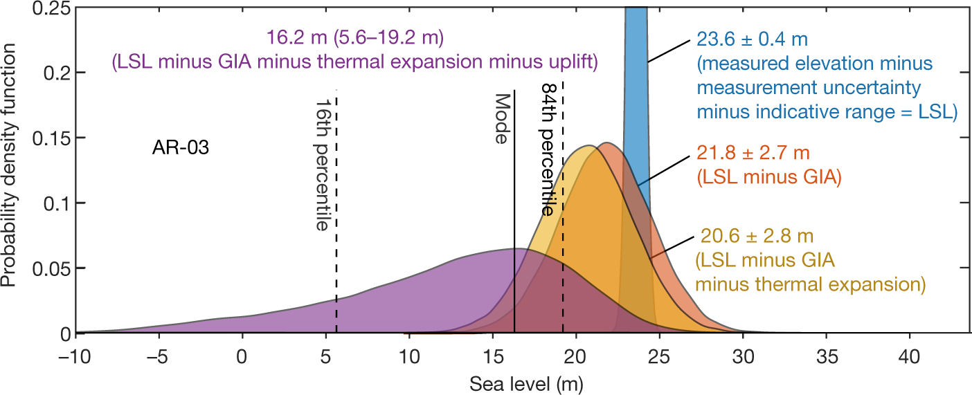
The paper I'll discuss is this one: Constraints on global mean sea level during Pliocene warmth (Onac, et al, Nature 574, 233–236 (2019)).
Currently, carbon dioxide accumulations are the highest recorded ever (although the record extends only to the mid 20th century), about 2.4 ppm per year and rising. We are currently reaching (or have reached) the annual minimum that comes every September. (It may end up being in October this year as the Northern Hemisphere's summer is extending with climate change.) The weekly low for this year was recorded at the Mauna Loa Carbon Dioxide Observatory for the week ending September 9, 2019, a reading of 407.96 ppm. The high for this year was recorded during the week ending May 12, 2019, when the reading was 415.39 ppm, the highest value ever recorded at Mauna Loa.
At 2.4 ppm per year, our current rising rate of increase, we should see 450 ppm in about 15 years, "by 2035" in the kind of language Greenpeace has been using for the last 50 years to describe when we will all live in a "renewable energy" nirvana powered solely be wind, solar, and all be driving electric cars, although in the old days, when I was a kid, that renewable energy nirvana was supposed to arrive "by 2000."
It didn't, but who's counting? We should do things on a faith basis, no, and only read Greenpeace "studies," because they always make you feel warm and fuzzy.
Warm, definitely. It's getting very hot these days. Fuzzy? I don't know. How does "fuzzy" feel?
The reason that this 450 number sticks in my mind, other than the 350 number about which Bill McKibben likes to talk, is the cited paper refers to a period, the Pliocene, which was relatively recent in geological history when carbon dioxide briefly was above 450 ppm. Let me jump the gun a little and post a figure from the paper before excerpting any text. Here it is, figure 3:

The caption:
Some text from the abstract, which should be open sourced:
From the paper's introduction:
Oxygen isotope ratios from benthic foraminifera10 paired with deep ocean temperature estimates have been used to approximate ice-volume-equivalent GMSL changes over the Pliocene11,12. While invaluable, these approaches are limited by uncertainties in the methodology and a number of factors (for example, post-burial diagenesis, long-term changes in seawater chemistry and salinity) that are poorly constrained and may bias the sea-level estimates3. Field mapping of palaeoshorelines has been a complementary approach...
A few other means of estimating sea level height are given. The authors however choose a new approach:
"Phereatic overgrowths on speleotherms" refer to deposits that form on stalactites and stalagmites when they go under water.
Table 1:

Some other pictures in the paper:
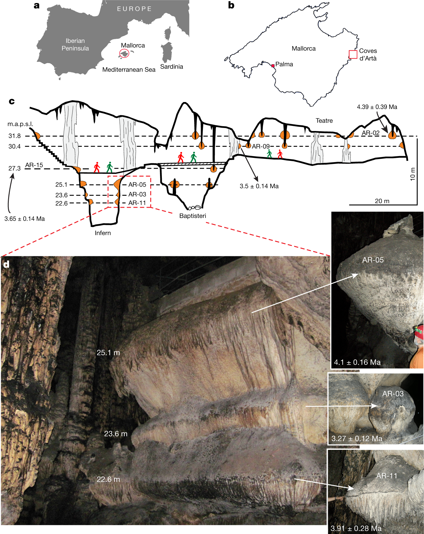
The caption:
The caption:
Figure 3 was produced here earlier.
An excerpt of the conclusion:
"m.a.p.s.l" is an unnecessary abbreviation of "meters above present sea level."
Don't worry. Be happy. It's not your problem. You'll be dead "by 2100" just like the people who bet the planet on so called "renewable energy," but happily will be dead when future generations will almost certainly not be able to achieve, because we have insisted blithely, that it will be easy for them to do what we could not do ourselves.
Most likely, the reality is that future generations, much as was the case for all generations before the 19th century will actually experience living by "renewable energy" the way those generations did: Then, as in the future I predict - may I be proved wrong - even more so than today, the bulk of humanity lived short, miserable lives of dire poverty.
History will not forgive us, nor should it.
I hope you enjoy the upcoming weekend.
Tuning element distribution, structure and properties by composition in high-entropy alloys.
The paper I'll discuss in this post is this one: Tuning element distribution, structure and properties by composition in high-entropy alloys (Zhu et al, Nature volume 574, pages 223–227 (2019))
Recently in this space, I referred to the presence of the relatively rare (but extremely useful) element palladium, a constituent of used nuclear fuel: Palladium is a fission product. In that post I referred to use of the element in thermoelectric devices, which convert heat directly into electricity, as in famous deep space spacecraft like Voyager, New Horizons and the spectacularly successful Cassini mission. I argue that similar (more efficient) thermoelectric devices can raise the thermodynamic efficiency of nuclear plants, thus accelerating the ease of addressing climate change by the only feasible approach to do so.
As of this writing, the price of palladium is about $54,000/kg at a kg scale.
Non-radioactive palladium can be isolated only from rapidly reprocessed nuclear fuels or those that are continuously reprocessed, which is possible for fluid phased reactors, such as those with salt based fuels or (my personal favorite because of extremely high neutronic efficiency) liquid metal fuels like the LAMPRE reactor which operated in the early 1960's at Los Alamos using a plutonium/iron eutectic. (Other plutonium eutectics are known.)
Separation would involve exploiting the volatility of ruthenium tetraoxide generated from extracted metal samples, and allowing the obtained ruthenium's 106 isotope to decay and harvesting the non-radioactive palladium-106 daughter.
Older nuclear fuels will contain the radioactive palladium isotope Pd-107, which is an isotope representing low risk, since it is a low energy pure ?- with no penetrating radiation, that will be diluted by, Pd-104, Pd-105, Pd-106, Pd-108, and Pd-110. This should allow for wide use of this palladium, if and only if the stupidity of some of the less educated, i.e. ignorant, people responsible for 7 million deaths per year from dangerous fossil fuel and biomass combustion waste is rejected in an effort to save humanity from itself.
(The worst kind of ignorance is deliberate ignorance expressed with a complete lack of shame and with some force, that is, Trumpian ignorance. I have been sparing myself from engaging people here who represent exemplars of this kind of ignorance. As this is an issue on a national scale, I often reflect on a lecture I saw by the neuroscientist - and anti-gerrymandering activist - Sam Wang in which he claimed that the best way to give lies credibility is to repeat and report them while trying to discredit them. This may, in my opinion, be true; it's at least worthy of consideration. I wish our national media believed that. I'm personally as tired of hearing drooled drivel from the so called "President of the United States" as I am of hearing the drivel of anti-nukes.)
Anyway, isotopes decaying either to stable palladium and including radioactive Pd-107, constitute, in direct fission, about 21.8% of fast fission events in plutonium-239, the fast fission of plutonium being the most desirable in terms of sustainability and foreclosing all energy mining (including uranium mining) for several centuries using uranium already mined. (The similar use of thorium already mined and dumped by the lanthanide industry might extend this period for additional centuries.)
Note this neglects neutron capture reactions, which depend in turn on the capture cross sections of the isotopes in the fast spectrum, but is useful as a first approximation.
World Energy Demand as of 2017, according to the 2018 World Energy Outlook put out by the EIA - the 2019 edition should come out soon - was 584.98 exajoules. To eliminate all energy mining by plutonium utilization would require the complete fission of about 7,300 tons of plutonium per year, and produce, therefore, about 1,500 tons of palladium per year. The availability of this element in such quantities would of course reduce prices and make use of the element more available, but at current prices, just for arguments sake, the value of this palladium would be about 82 billion dollars.
As for the radioactivity, neglecting neutron capture, and also neglecting the option of separating the 106 isomer, about 14.7% of the total palladium would be radioactive palladium-107. The long half life of Pd-107, 4.5 million years, yields a fairly low specific activity, about 0.4 millicuries per gram for the pure isotope, and, representing 14.7% of the total palladium, even less, 0.075 millicuries, or about 75 microcuries. As a pure beta emitter with low energy beta (0.987 keV) in a self shielding situation, it is hard to imagine than an alloy containing this palladium would exhibit any health risk to persons using it as a structural alloy, which is what the cited paper is all about.
Note that the alloy discussed therein would represent even further dilution of any Pd-107 related radioactivity, to even more meaningless levels, with the specific activities listed above reduced by a factor of five.
From the abstract:
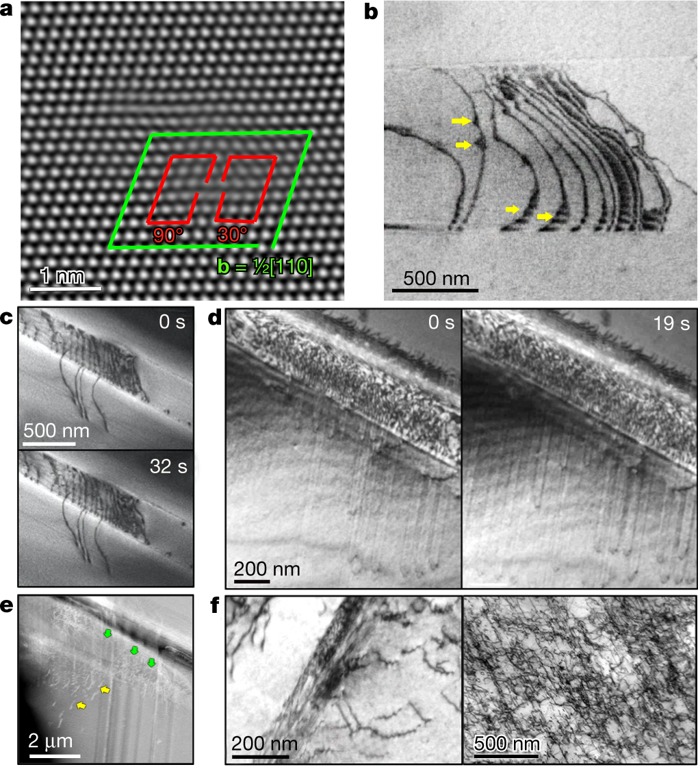
...These deformation mechanisms in the CrFeCoNiPd alloy, which differ markedly from those in the Cantor alloy and other face-centred cubic high-entropy alloys, are promoted by pronounced fluctuations in composition and an increase in stacking-fault energy, leading to higher yield strength without compromising strain hardening and tensile ductility. Mapping atomic-scale element distributions opens opportunities for understanding chemical structures and thus providing a basis for tuning composition and atomic configurations to obtain outstanding mechanical properties.
(The abstract is probably open sourced.)
From the full paper's introduction:
Some pictures from the paper:
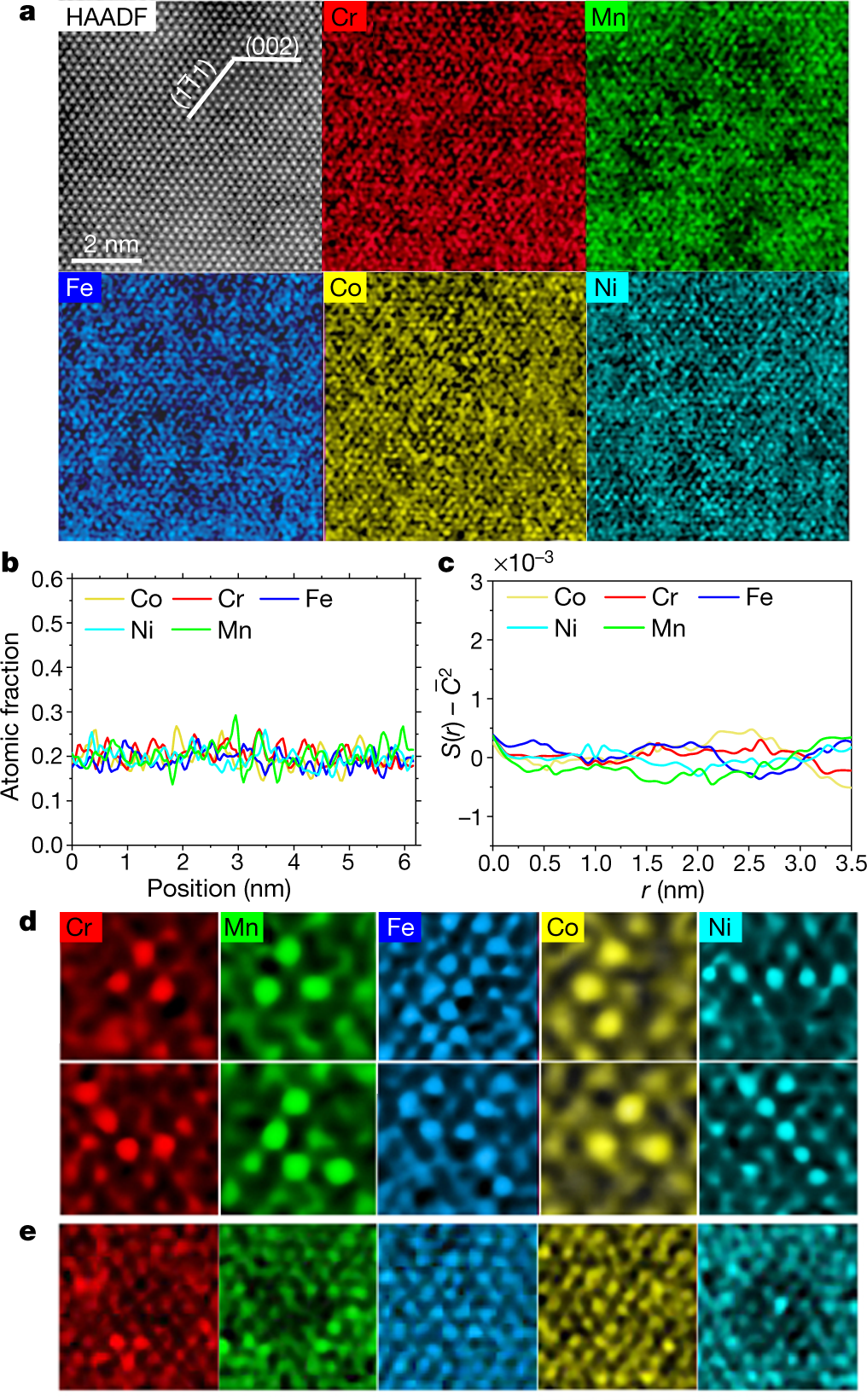
The caption:
HAADF refers to atomic-resolution high-angle annular dark field transmission electron microscopy (TEM), a techiniq my son about which probably knows the details. (I don't.) EDS refers to Electron Dispersive Spectroscopy.
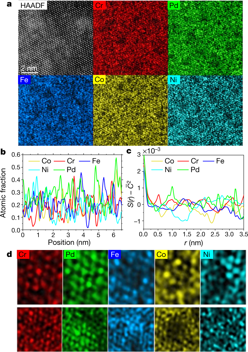
The caption:
Superscripts and lines over symbols are displaced in these captions because of the limits of the DU editor, but one can get the idea.
 ?as=webp
The caption:
The "money" picture:
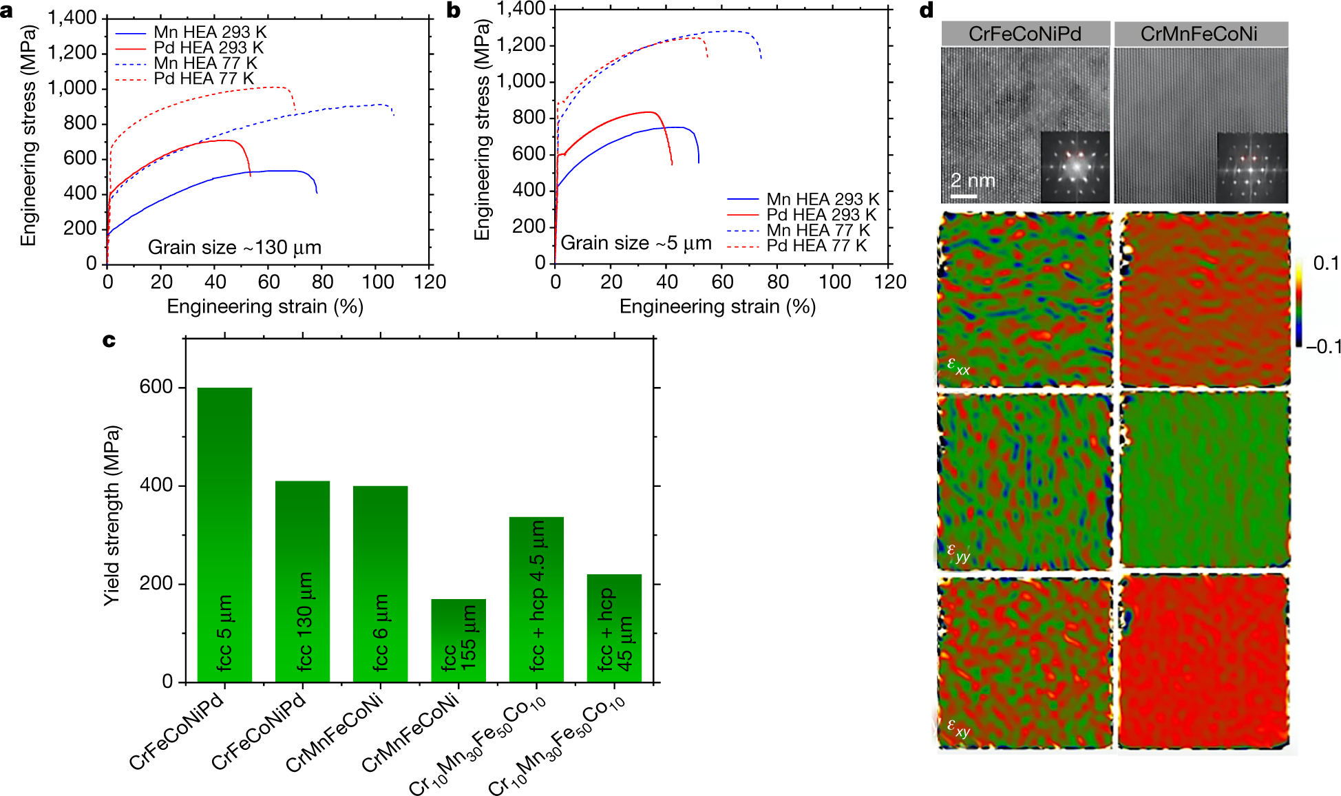
The caption:
The paper reports the temperature treatment of these alloys, but not mechanical strength at these temperatures:
Perhaps therefore with appropriate thermal barrier coatings, these alloys may be usable in high temperature turbines, where strain resistance, strength, is important. The engineering details are beyond the scope of this post, but I would like to see Brayton type nuclear heated turbines with a carbon dioxide working fluid operating at around 1400 °C for the purposes of reducing carbon dioxide. Such a system might exhibit extremely high exergy.
My son has a long weekend coming up, and will be visiting us at home. I'm looking forward to discussing this paper with him.
I wish you a pleasant day tomorrow.
Dealing with 11 Million Tons of Lithium Ion Battery Waste: Molten Salt Reprocessing.
The paper I'll discuss in this post is this one: Low-Temperature Molten-Salt-Assisted Recovery of Valuable Metals from Spent Lithium-Ion Batteries (Renjie Chen et al, ACS Sustainable Chem. Eng. 2019, 7, 19, 16144-16150)
There is, in the United States, about 75,000 tons of used nuclear fuels, generated in the United States, with 100% of the materials therein being valuable and recoverable. All of this material, called "nuclear waste" by people who have never opened a science book in their lives but nevertheless like to assert their ignorance loudly - as in the idiotic comment "Nobody knows what to do with 'Nuclear Waste'" - is located in about 100 locations, where it has been spectacularly successful at not harming a single soul.
If one doesn't know what to do with so called "nuclear waste," it's not like one is even remotely qualified to understand anything about nuclear energy because it is obvious that one has not opened a reputable science book in one's life. One's ignorance it obvious in this case, but it's not like, in Trumpian times, people are unwilling to make sweeping generalizations and pronouncements on subjects about which they know nothing.
Irrespective of the ignorance of anti-nukes, it is a shame to let these valuable materials, the only materials with high enough energy density to displace dangerous fossil fuels, go to waste, and I have spent about 30 years studying their chemistry, coming to the conclusion that the ideal way to recover the valuable materials therein is via the use of molten salts in various ways.
There are, by the way, as has been discovered in my lifetime, potentially an infinite number of such salts, and they can be finely tuned for any purpose one wishes.
By contrast to used nuclear fuel, electronic waste is widely distributed; its toxicology is not understood by the people who use it, including scientifically illiterate anti-nukes who run their computers parading their ignorance, without a care in the world about what will become of the electronic waste in their computers, their electric cars, their solar cells, their inverters, and the television sets in front of which they evidently rot their little brains. Electronic waste is not only widely distributed; it is massive and growing rapidly in volume, because of the dangerous conceit that so called "renewable energy" is "green" and "sustainable," neither of which is true.
The lithium ion battery was discovered in 1980 According to the paper I'll discuss shortly, by 2030 the total mass of lithium batteries that have been transformed into potential landfill will be 11 million tons. (I'll bold this statement in the excerpt of the paper's introduction below.) This means that each year, on average, since their discovery, 282,000 tons of waste batteries are taken out of use, about 370% of the mass of nuclear fuel accumulated over half a century.
It is only going to get worse with the bizarre popularity of electric cars, which dumb anti-nukes, with their Trumpian contempt for reality, imagine are all fueled by solar cells and wind turbines, even though solar cells and wind turbines, despite the expenditure of trillions of dollars on them have only resulted in climate change accelerating, not decelerating, since a growing[ proportion of the electricity on this planet is generated by dangerous fossil fuels, not so called "renewable energy."
It is difficult to recycle distributed stuff, and of course, it takes energy even if one can find an electronic waste recycling center, to drive to it, never mind the energy required to ship it to some third world country where the toxic materials therein will be less subject to health scruples. Inevitably, much electronic waste ends up in landfills, where it is forgotten, at least until the health effects begin to appear.
From the paper:
State-of-the-art techniques for recycling of spent LIBs have been reviewed in several studies.(2,6?10) Generally speaking, existing recovery strategies can be divided into pyrometallurgical, direct generation, and hydrometallurgical processes. Pyrometallurgical processes are usually undertaken at high temperature, resulting in relatively high energy consumption.(11?13) The alloyed product and residue require further processing to obtain high-purity products.(14) Direct generation has stringent requirements for the purity of the feed and is not appropriate for recycling materials containing large amounts of impurities.(15) In contrast, hydrometallurgical methods have obvious advantages, including high recovery efficiency of valuable metals, mild reaction conditions, and environmentally friendly conditions. These advantages make hydrometallurgical methods a preferable and promising approach for disposing of spent LIBs; however, the inorganic(16?19) and organic(14,20?22) acids used in hydrometallurgical processing may cause secondary pollution, such as acidic waste waters and production of toxic gases (Cl2, SO3, and NOx) during the leaching process, which are threats to the environment. Therefore, developing a method to reduce acid consumption, decrease the emissions of the secondary pollution, and increase recovery efficiencies of metals is critical. A salt-assisted calcination method has recently been proposed that avoids the above issues and increases recycling efficiency.(23)
Salt-assisted calcination has become widely used as a metal-recovery method for waste materials due to its high reactivity, high volatility, low melting point, and high solubilities of salts.(23?30) In addition, the solid salt agents used are generally environmentally friendly, and the process has simple operation and low-cost equipment.(28) For example, Liu et al.(31) reported a vacuum chlorinating process for simultaneous sulfur fixation and lead recovery from spent lead-acid batteries using calcium chloride (CaCl2) and silicon dioxide (SiO2) as reagents. Dang et al.(23) proposed a chlorination roasting method to recycle lithium from a pyrometallurgical slag using three chlorine donors; namely, NaCl, AlCl3, and CaCl2. These findings showed that it is possible to recover metals through salt-assisted roasting, but the reaction temperature of these solid salt fluxing agents is quite high.
In this work, we developed a combination of low-temperature ammonium salt roasting and water leaching to efficiently and environmentally recover valuable metals from spent LIBs. NH4Cl, a nontoxic and noncorrosive solid chlorinating agent, can be decomposed to NH3 and HCl gases above 230 °C; (32) the introduction of NH4Cl as a chlorinating agent into the calcination process can therefore destroy the crystal structure of LiCoO2 and enable precipitation of Li and Co. Owing to the high solubilities of the chloride salts, the metals are recovered by water leaching after chlorination. The effects of various parameters on recovery efficiencies of Co and Li, including calcination temperature, time, and mass ratio of LiCoO2 to NH4Cl, were systematically investigated. The mechanism underlying the low-temperature molten-salt-assisted recovery process is discussed in detail. The method was proven by efficiently recovering valuable metals from LiMn2O4 and LiCo1/3Mn1/3Ni1/3O2 spent LIBs. This study presents an environmentally friendly and efficient method for recovery of metals from mixed cathode materials of spent LIBs.
I have bolded the information described above. Reference 4 is here: Burgeoning Prospects of Spent Lithium-Ion Batteries in Multifarious Applications (.Natarajan, S.; Aravindan, V. Burgeoning Prospects of Spent Lithium-Ion Batteries in Multifarious Applications. Adv. Energy Mater. 2018, 8 (33), 1802303– 1802319)
One can question, if one wishes, how environmentally "friendly" a process requiring a temperature of 230 °C really is, there is certainly no efficient and scalable way to do this with so called "renewable energy" on which all our battery worshipping types have bet the planetary atmosphere, a bet we are losing at great cost to all future generations.
No matter. I personally believe that to the extent that we can close material cycles, not just for nuclear fuels but for everything, not limited to carbon either, the less odious we will appear in history, although, as I often say, history already will not forgive us, nor should it. I own lithium batteries, and to the extent the materials in them can be recovered, so much the better, fewer modern day African children will need to dig cobalt for example.
Here are the chemical reactions and the equations for thermodynamic values in this process:


Note that one of these reactions is the oxidation of ammonia to nitrogen gas using chlorine gas. Almost all of the world's ammonia is produced from hydrogen produced using dangerous natural gas, although one could have read over the last five decades or so, and can still read, lots of increasingly delusional claims that hydrogen "could" be produced by so called "renewable energy." After half a century of such rhetoric, almost none of it is.
The oxidation of ammonia by chlorine is thus an energy penalty reaction.
Before touching figure two which graphically obviates the thermodynamic penalties for recycling these putative energy storage devices, let me offer the cartoon of the "flowsheet" which is nice art:

The caption:
The thermodynamics, reactions being viable when the Gibbs free energy, ?G, is below the zero line:

The caption:
A few more graphics:

The caption:

The caption:

The caption:

The caption:
Verification of the process is described:
From the conclusion of the paper:
There is very little discussion of the electrolytes and what to do with them in this paper, but no matter. This process seems fairly sustainable with the use of clean heat, readily accessible with nuclear energy.
To the extent we can close materials cycles, even given the logistics and energy requirements of recovering distributed materials, the better we can do at ameliorating the contempt in which history will hold us.
Have a nice evening.
The Toxicity of Soy Biodiesel Combustion Waste and Petroleum Diesel Combustion Waste Compared.
The paper from the primary scientific journal I'll discuss in this post is this one: Soy Biodiesel Exhaust is More Toxic than Mineral Diesel Exhaust in Primary Human Airway Epithelial Cells (Katherine Landwehr et al, Environ. Sci. Technol. 2019 53 19 11437-11446)
In general, I am a critic of so called "renewable energy" - although, albeit some ago, I supported it - since it didn't work, isn't working and won't work to address climate change or the other massive environmental and health consequences of fossil fuels. To me, betting the future of humanity on this unworkable, & failed strategy is nothing more than a de fact acceptance of the death toll associated with dangerous fossil fuels.
This said, since we have destroyed the planet with our wishful thinking about so called renewable energy, I try to ameliorate my knowledge of the disgrace that my generation has brought on itself, by imagining ways that future generations might restore anything left to restore, in particular, the atmosphere. The energy requirements, if only because of the entropy of mixing, of removing carbon dioxide from the air are enormous, and so I turn a less jaundiced eye on biomass than I do on say, wind or solar energy, both of which are useless in any case, and both of which will involve the destruction of huge amounts of the already vanishing wilderness for mines and industrial parks.
The use of biomass, of course, extends way back. Humanity only abandoned biomass as its primary source of energy beginning in the early 19th century, because most people lived short, dire, lives in poverty, even more so than today.
The current use of biomass is still killing people as it did back then, although the death toll associated with it is slightly superseded by the death toll associated with dangerous fossil fuel waste.
Dangerous fossil fuel waste and dangerous biomass combustion waste are responsible for about 7 million deaths per year, something I often state when confronted with an ignoramus chanting his or her ignorance about so called "nuclear waste."
Some biofuels are better than others, of course. Back in the 1970's, when I was a dumb-assed anti-nuke,with effectively no education (and no access to the primary scientific literature) - when as dumb as the assholes here who chant about so called "nuclear waste" (about which they know zero since they are spectacularly unacquainted with the contents of science books) - I thought Jimmy Carter's ethanol program was a great idea.
It lead, of course, to the complete destruction of the Mississippi River Delta's ecosystem, because of phosphorous and nitrogen run-off, and it placed responsibility for selecting the candidates for Presidents of the United States in the hands of Iowans, a group of people who do stuff like vote for an orange racist pervert chanting, similar to dumb anti-nuke chants in their depth of thought - about "Making American 'Great' Again" by turning it over to the kind considerations of Vladimir the Giggler, the imperialist fascist running Russia.
So much for corn ethanol.
In the past, I've thought better of biodiesel, and once even gave serious thought to making some myself. As is well known, at least by people who give a shit, "renewable energy portfolio standards" - many addressed by biodiesel in Germany, has lead to the destruction of huge swathes of the South East Asian rainforest to make palm oil plantations.
Biodiesel, of course, is the esters of plant lipids (although animal fat has also be used) produced by transesterification of the glycerol found in natural lipids with methanol (usually) and more rarely ethanol. Methanol is usually produced by the partial oxidation of dangerous natural gas.
At least, I thought, somewhat as a consolation to this reality is that at least biodiesel burned cleaner than petroleum diesel and at least, I thought, it was something of a closed carbon cycle. The latter point of course, needs consideration of the carbon content of a rain forest in comparison to a palm oil plantation, but the former, which I assumed to be the case until I came across this paper last night, also turns out to be questionable.
From the paper's introduction:
Most previous studies comparing mineral diesel and biodiesel combustion have found that biodiesel exhaust contains more toxic gases such as nitrogen oxides and a greater proportion of smaller particles which, when inhaled, penetrate deeper into the lungs.(3,4,8,9) Despite the potentially more toxic effects of biodiesel exhaust, most studies comparing biodiesel with commercial mineral diesel rather focus on fuel economy and engine wear or the physicochemical differences between the exhausts.(4,9) Few studies compare the health effects with exhaust exposure.(7,10,11) Such studies primarily use the Ames mutagenic assay(12,13) or immortalized cell lines(8,14) and the majority of the studies only focus on the cytotoxic and mutagenic potential of the particulate matter, ignoring the effects of the gaseous components of the exhaust entirely.(7,15) Particle concentrations are also rarely relevant to real-world exposure levels, often being far too concentrated to simulate a realistic dosage.(15) In addition, in in vitro-based studies, the cell lines used are not always human, or even derived from respiratory tissues.(3,16) This brings into question their relevance in human exposure studies where the main exposure route through inhalation of the exhaust means that the respiratory epithelium is among the first tissue exposed and thus likely to be among the most effected. Immortalized cell lines also negate genetic variability and are limited in how accurately they can model normal human tissues.(17)
If exhaust is typically inhaled, health complications can occur in the respiratory,(18,19) circulatory,(20) and immune systems.(21) Of concern, inhalation of ultrafine exhaust particles has been correlated with exacerbation of childhood asthma,(22) and associations between air pollution from major roads and decreased lung function in children have been identified.(23,24) This suggests that children may be at greater risk from adverse health effects caused by exhaust exposure. This is unsurprising as children breathe faster than adults and have higher ventilation to lung surface area/body weight ratios,(25) meaning that over the same period of time, they are exposed to a larger dosage of exhaust than adults.(25,26) In addition, the respiratory and immune systems of children are still developing and insults, such as exposure to large concentrations of exhaust, are known to have lifelong consequences.(23,27,28) Despite this, the effect of exposure to biodiesel exhaust has not yet been studied in children.
Because of the paucity of information in this setting, we tested the hypothesis that the soy biodiesel exhaust would contain a greater proportion of ultrafine particles and more oxides of nitrogen and thus exposure would result in more pronounced effects on the airway epithelium. To test this, we exposed primary human airway epithelial cells from young healthy volunteers to whole exhaust from a diesel engine fueled by either pure mineral diesel, a 20% blend of soy biodiesel with mineral diesel, or pure soy biodiesel. Physicochemical exhaust properties were recorded and 24 h post exposure, cells were analyzed for a variety of health effect end points.
The authors obtained epithelial cells from children, cultured the cells, and exposed the cells (not the children) to the exhaust of petroleum diesel and biodiesel.
The fuels were burned in a test engine to produce the exhaust. The test engine was a Yanmar L100V engine, a single cylinder small diesel engine for industrial use.
The exhausts were tested using standard equipment like for which the Volkwagen company programmed defeating software into its "green" cars.
These graphics show the results:

The caption:
The caption:


The caption:

The caption:
A little on cytokines, since this topic may be somewhat obscure:
Cytokines are small signalling proteins, very much involved with the immune system. Under certain conditions, they can be pathological in the sense of producing inflammation and (as implied here) cell death.
Not necessarily, good news, this paper, I think.
It is possible, still, I think, to utilize biomass safely, particularly fast growing biomass like algae. This approach can capture carbon dioxide because of the inherent ability of life forms to replicate and expand surface area. The use of such biomass were it to be done safely, however, in contrast to simple chemical modifications like transesterification, would involve supercritical water oxidation (SWO) or pyrolysis, subjects about which I've written here and elsewhere.
This paper, nevertheless, suggests that in the case of a particular biofuel, soy biodiesel, operating in a particular type of diesel engine, a one cylinder portable diesel, the "renewable case" is actually worse than the dangerous fossil fuel case, which is not to excuse the dangerous fossil fuel case.
The current issue of Environmental Science and Technology, a scientific journal I read almost religiously, and have been reading for many, many years is pretty focused - it's nice to see this at long last - on some questioning of the common "renewable energy" assumptions, and myths one being whether "renewable energy" is actually "renewable." I especially enjoyed the paper I found yesterday about which I posted. It was about how a tiny country, an offshore oil and gas drilling hellhole, that likes to put "renewable energy" lipstick on its fossil fuel pig, will most likely not be able to sustain its wind energy program because of material considerations. The same Danish research group published in the same issue, a detailed analysis of the platinum mass flows associated with so called "renewable energy" and the "100% renewable by 2050" bullshit we hand out with our continuing contempt for future generations.
Nevertheless, the nice thing about reading scientific journals is that, even if they go off on a trend that is less than fruitful or even wise, reality ultimately leads to self correction.
Published science can be wrong, or more mildly, mistaken, but science that is either, is self correcting, because in science, facts matter. More and more, I'm seeing questions rising about so called "renewable energy," and this is a good thing, because a process which cannot stand questioning does not deserve to proceed, particularly at risk to all humanity.
It is, by the way, no matter how much chanting and sloganeering goes on, a fact that the death toll from dangerous fossil fuel and biomass waste - about which many people here (I'm referring to rote anti-nukes of the type populating my ignore list) couldn't care less - is enormous, while the death toll from so called "nuclear waste" (about which they chant in a phenomenally ignorant fashion) is trivial, despite all the coal and oil burned to run computers to complain about "nuclear waste." So called "nuclear waste" hasn't killed anyone in this country in half a century. Air pollution, by contrast, never stops killing.
Betting the planet on so called "renewable energy" which hasn't worked, isn't working, and won't work, is the equivalent of announcing that one accepts the death toll associated with air pollution (not to mention climate change) and thinks it trivial and also that one thinks that destroying the entire planetary atmosphere, the climate, and all the ecosystems dependent on the climate and the atmosphere is acceptable because one is mindless enough to engage fetishes involving the dopey selective attention that thinks that Fukushima was the end of the world. It wasn't. This is a fact.
One of the interesting facets if one is to ponder this quality of thinking, which is Trumpian the depth of its delusion and the inherent gaslit (literally) lies such thinking involves, is the amusing fact that it is easy to insert one's head very far up one's ass if one's brains are soft, small, and largely empty.
All joking aside, dangerous fossil fuels must be banned. It can be done, but not so long as we surrender to the application of deliberate ignorance. Fuels based on food products won't do it any more than wind turbines, electric cars and solar cells will do it.
Have a nice day tomorrow.
Resourcing the Fairytale Country with Wind Power: A Dynamic Material Flow Analysis
Given my hostility to the wind industry, said hostility stemming from the belief that it is not only ineffective, but also unsustainable, let me state that the title for this post is identical to the title of the paper I will discuss in it, and that three of the authors of this scientific paper work in academic institutions in that offshore oil and gas drilling hellhole, Denmark, despite having names with Chinese origins.
The paper in question is this one: Resourcing the Fairytale Country with Wind Power: A Dynamic Material Flow Analysis (Liu et al, Environ. Sci. Technol. 2019, 53, 19, 11313-11322)
The introduction, indicating that it focuses on the Danish case, which I hold up as an indicator that so called "renewable energy" isn't working and won't work, particularly because Denmark is a small country jutting into the North Sea, which it has laced with wind turbines and offshore oil and gas rigs:
For example, Denmark, a pioneer in developing commercial wind power since the 1970s’ oil crisis, has built up an energy system of which already about 48% of electricity is from wind in 2017.(14,15) The intermittent yet abundant wind energy in Denmark will continue to play a major role for achieving the Danish government’s ambition to have a “100% renewable” energy system by 2050.(16,17) Understanding potential resource supply bottlenecks, reliance on foreign mineral resources, and secondary materials provision is, therefore, an important and timely topic for both the Danish wind energy sector and Denmark’s energy and climate policy.
Construction and maintenance of wind power systems needs large quantities of raw materials mainly due to large-scale deployment of wind turbines and infrastructure on land or at sea.(18) In particular, two rare earth elements (neodymium and dysprosium) mainly used in permanent magnets have raised special concerns in the wind energy sector(10,19,20) due to overconcentration of rare earth’s supply in China,(21) sustainability of upstream mining and production processes,(22) and complexity of wind turbines’ supply chain.(23) Moreover, the wind energy sector also faces increasing challenges in both meeting future demands for several base metals (e.g., copper used in transmission(18)) and managing mounting end-of-life (EoL) materials (e.g., glass fiber in blades(24?26)) arising from decommissioned wind turbines.
A variety of methods have been used to translate wind energy scenarios into material demand. If the annual newly installed capacity of wind turbines is given, its associated material demand is often directly determined by material intensity per capacity unit.(5,8,9,27?30) If annual installed capacity is not given, its associated material demand can be derived from a life cycle assessment (LCA)-based input–output method,(31) economic model,(32) or dynamic material flow analysis (MFA) model.(6,11,20,25,30,33?36) The dynamic MFA model has been increasingly used to explore material requirements of wind energy provisioning on a global scale,(6,11,30,33,34) country scale (e.g., the US,(20) France,(25) and Germany(35)), or country scale with a regional resolution.(36) The principle of mass balance constitutes the foundation of any MFA, so that the annual newly installed capacity (“inflow”) and annual decommissioned capacity (“outflow”) of wind turbines are driven by their lifetime and the expansion and replacement of the installed wind power capacity (“stock”),(20,36) which has also been widely used in other anthropogenic stock studies.(37)
However, the current practice of modeling raw material requirement or secondary material availability in different wind energy technologies generally overlooks the hierarchical, layered characteristics of wind power systems. This is important because materials embedded in a technology system are usually distributed in its subsystem or subcomponents with varying compositions and recycling potentials.(38,39) In the case of wind power systems, materials employed in a wind turbine are distributed in its subcomponents such as rotor, tower, and nacelle, and their mass is largely determined by the turbine size (e.g., rotor diameter or hub height) and capacity.(13,40) These constraining factors and their leverages on the sustainability and resilience of the wind energy provisioning should be fully examined. Such information would enable wind turbine manufacturers, material suppliers, recyclers, end users, and policy makers to plan their material-related policies with a comprehensive understanding on a range of important aspects related to wind energy provisioning, such as secondary material supply, technological development, and material efficiency.
Here, we developed a component-by-component and stock-driven prospective MFA model to characterize material requirements and secondary material potentials of different Danish wind energy development scenarios. Based on two datasets that cover a range of microengineering parameters (e.g., capacity, rotor diameter, hub height, rotor weight, nacelle weight, and tower weight) of wind turbines installed in Denmark and worldwide, we established empirical regressions among these parameters in order to address the size scaling effects of wind turbines.
Some graphics:

The caption:

The caption:

The graphic refers to the Danish Master Register of Wind Turbines, which I have often appealed to in this space, at least in the E&E forum where I used to write from time to time.
The caption:
This graphic cleanly draws out the number of wind turbines that will become landfill as the wind industry, um, "expands."

The caption:
By the way, the "hydrogen" scenario has been under discussion with tons and tons and tons of wishful thinking applied to it. A pilot program on the Norwegian island of Utsira, which generated a huge internet hoopla, and was designed to power ten homes, was finally reduced to "lessons learned." The entire project generated many orders of magnitude of hype as opposed to, um, hydrogen.
Some useful text from the paper before examining the dysprosium and neodymium cases in graphics:
Figure 5 assembles the results of material requirements (inflows) and potential secondary materials supply (outflows) during 2018–2050 under the six scenarios. Several key observations on the trends of inflows and outflows are detailed below.
•The inflows of bulk materials (concrete, steel, cast iron, nonferrous metals, polymer materials, and fiberglass) under the hydrogen, IDA, and wind scenarios will increase by 413.31, 211.91, and 328.83%, respectively. Meanwhile, the outflows of bulk materials will increase by 52.90, 49.86, and 33.15%, respectively. On the contrary, the inflows of bulk materials will increase at a slower rate under the fossil and biomass scenarios or fall slightly under the biomass+ scenario. Meanwhile, the outflows of bulk materials will decrease by 23.71, 15.98, and 37.76%, respectively.
•The inflow of neodymium under the hydrogen, IDA, and wind scenarios will climb to 14.50, 12.36, and 11.15 tonne year–1, respectively. Meanwhile, the outflow of neodymium will swell to 5.64, 5.71, and 4.98 tonne year–1, respectively. On the contrary, the inflow of neodymium will decrease at first and increase to 3.78 and 4.28 tonne year–1 under the fossil and biomass scenarios, respectively, or decrease to 2.46 tonne year–1 under the biomass+ scenario; meanwhile, the outflow of neodymium will climb up and stabilize at a certain level under the fossil (3.07 tonne year–1), biomass (3.34 tonne year–1), and biomass+ (2.60 tonne year–1) scenarios.
•A similar trend is observed in the inflow and outflow of dysprosium. The inflow of dysprosium under the hydrogen, IDA, and wind scenarios will eventually climb to 1.73, 1.48, and 1.33 tonne year–1, respectively. Meanwhile, the outflow of dysprosium will simultaneously grow to 0.67, 0.68, and 0.59 tonne year–1, respectively. On the contrary, the inflow of dysprosium will decrease at first and increase to 0.451 and 0.51 tonne year–1 under the fossil and biomass scenarios, respectively, or decrease to 0.29 tonne year–1 under the biomass+ scenario; meanwhile, the outflow of dysprosium will climb up and stabilize at a certain level under the fossil (0.37 tonne year–1), biomass (0.40 tonne year–1), and biomass+ (0.31 tonne year–1) scenarios.
•The aforementioned observations indicate that, in the case of both bulk materials and critical materials, the gap between their inflow and outflow will be enlarged under the hydrogen, IDA, and wind scenarios, and it will still be enlarged but to a lesser degree under the fossil, biomass, and biomass+ scenarios.
Nowhere mentioned here is the nuclear case, since we're in fairy tale land and there's no purpose to discussing things that might actually work.
Some mass flows under the scenarios explored in this paper:

The caption:
From the text:
Of course this depends on Denmark changing the way it currently handles it's waste, which is to ship it to countries including those with lower standards of living than Danes:
And of course, there's no indication that circularity will be economically or technologically viable, but of course, it's a good idea to demand that future generations do what we are clearly incapable of doing ourselves, the old "by 2050" scam that's applicable in this paper because of the Danes claim that they will be 100% renewable "by 2050" - when most of the government administrators making this claim will be dead.
One last graphic:

The caption:
From the conclusion to the paper:
If any of this remotely troubles you, don't worry, be happy. It's not your problem; it's the problem of every living thing that will come after us.
History will not forgive us; nor should it.
Have a nice evening.
Steel Flows in the United States.
The paper I'll discuss in this brief post is this one: Mapping the Annual Flow of Steel in the United States (Yongxian Zhu, Kyle Syndergaard and Daniel R. Cooper, Environ. Sci. Technol.2019, 53, 19, 11260-11268)
The production of steel is coal dependent, and all the hand waving and fantasies in the world about the death of coal will not change this fact in the immediate future. Personally I believe that it is technologically feasible to displace coal in steel making, but not using steel intensive industries like, say, the wind industry, although the effort to make it significant - which will fail because of the simple laws of physics - will uselessly consume a lot of steel for no good purpose.
From the paper's introduction, verifying the fact of the GHG intensity of steel:
Realization that steel production must decrease if emission targets are to be achieved has helped lead to new research areas under the banners of “material efficiency”(5) and “circular economy”,(6) both aimed at reducing emission-intensive material production. Researchers in these new areas require a detailed material map in order to identify opportunities.
Unlike in the developing world, U.S. per capita steel stocks plateaued around 1980. The stock saturation level has been estimated at 9.1–14.3 t/capita.(7?9) Per capita stocks are expected to saturate in much of the developing world to a level similar to those in the U.S. by the late 21st century.(10,11) Therefore, the derived U.S. consumption pattern may represent a population-scaled surrogate model of the future global state.
I'll just cut to two of the informative graphics, one of which is a Sankey diagram of US steel flows, which, to utilize, one may need to utilize expanded views and rotation tools:

The caption:

The caption:
It is notable that the United States throws away more steel than it produces from pig iron and that amount of steel consumed for transportation is double that of the rest of the world, even if we love to declare ourselves "green" in contrast to say, China:
In a closed carbon cycle world, which I freely admit would be energy intensive, one can imagine the separation of impurities like copper might be conceivable.
Interesting paper, I think.
I trust you're having a wonderful afternoon.
Profile Information
Gender: MaleCurrent location: New Jersey
Member since: 2002
Number of posts: 33,516